Warehousing Operations

Optimize Warehouse Value Added Services with Python

Use Linear Programming to Increase your Production Capacity for the Final Assembly of Luxury Products

Most of the challenges faced by Distribution Centers (DC) handling Luxury Products, Garments or high-value goods are during the Inbound Process.

We will take the example of a DC storing imported Luxury Bags, Garments and Shoes that need:

Machine 1 — Anti-theft tag: Put a self-alarm tag to protect your goods against theft in the store

Example of Anti-theft tag — (Image by Author)

Machine 2 — Labelling: print labels in the local language and perform label sewing

Machine 3 — Kitting & Repackaging: transfer your goods into the sales packaging and add Gift With Purchase (GWP), Individual Note or Certificate of Authenticity

Example of packing with Gift with purchase and certificate — (CAD Model by Author)

After completing these 3 steps, your goods are ready to be put away in the stock area and are awaiting pickup for shipping to their final destinations (Store).

If your capacity for items handled by day is too low, this process can quickly become a major bottleneck.

💌 New articles straight to your inbox for free: Newsletter

Problem Statement

Scenario

You are an Inbound Manager of a Distribution Centre (DC) for an iconic Luxury Maison focusing on Fashion, Fragrance and Watches.

You have received 600 prêt-à-porter sets (Ready-to-wear) including:

1 Female dress that requires Label Sewing and Re-packing
1 Handbag that requires Label Sewing, an Anti-theft tag and Re-packing
1 Leather Belt that requires an Anti-theft tag, Label Sewing and Re-packing

Because they are sold together, they need to be ready at the same time and co-packed together before shipping to stores.

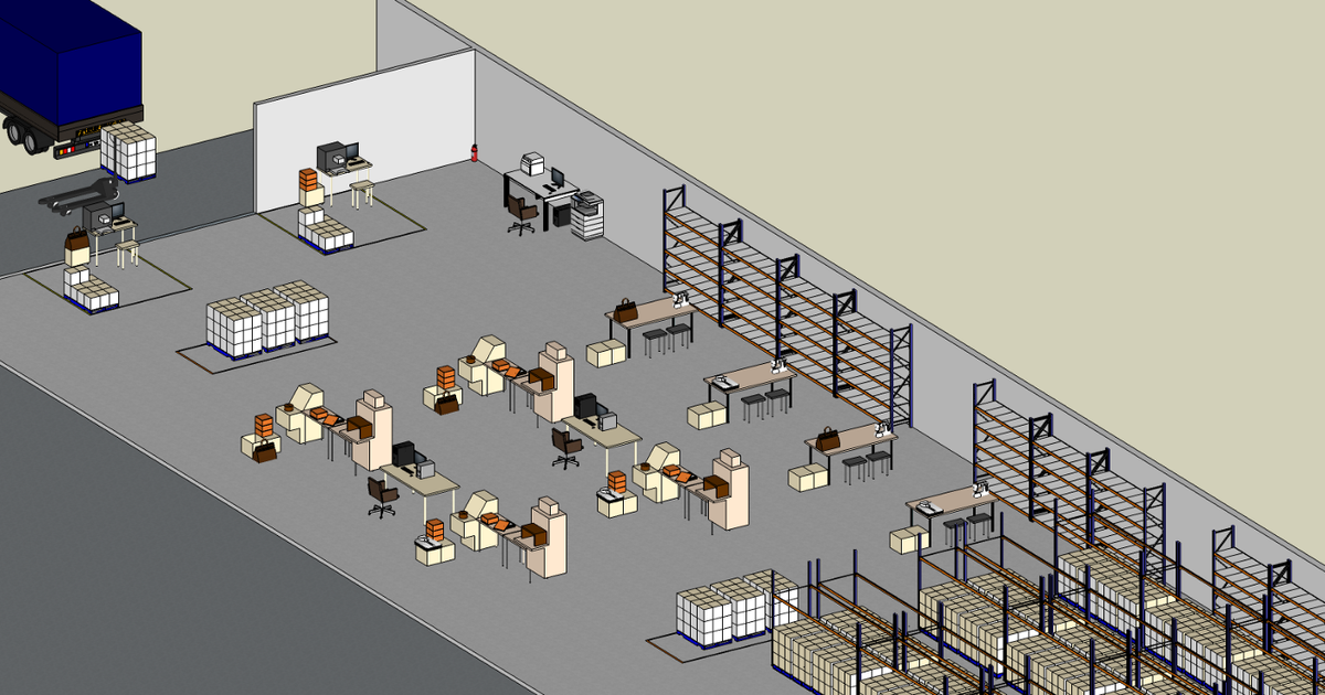
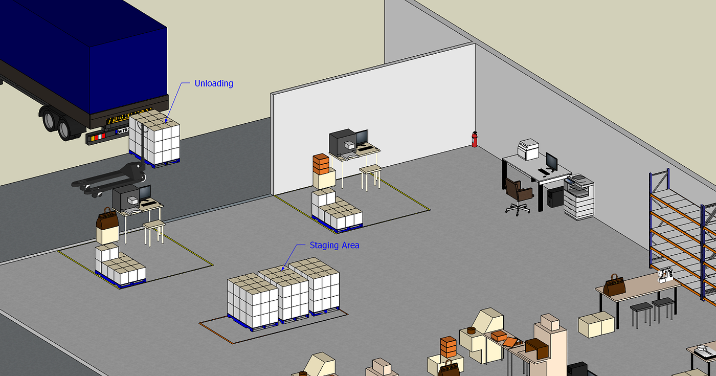
The inbound team is unloading pallets from the truck and putting them in the staging area

Step 1: Unloading and transfer of the pallet to the staging area — (CAD Model by Author)

Machine 1: Anti-theft tag — an operator put an anti-theft tag on each bag and belt

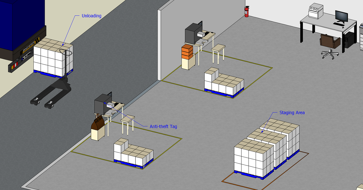
Step 2: 2 workstations where operators put an anti-theft tag on each Handbag and Belt — (CAD Model by Author)

Machine 2 — Labelling: after printing in a dedicated area, labels are sewed on belts, handbags and dress

Step 3: 4 workstations where operators perform label sewing — (CAD Model by Author)

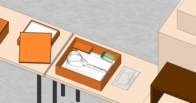
Machine 3 — Kitting & Repackaging: for each item, you need to add a certificate of authenticity, plastic protection and perform fine packing

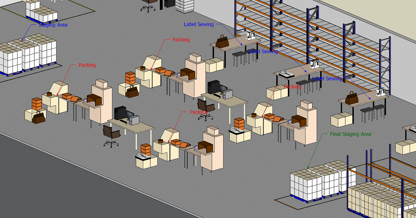
Step 4: 4 workstations where operators perform re-packaging — (CAD Model by Author)

After repackaging, goods are transferred to a final staging area to await shipping.

Objective: Reach maximum productivity of sets assembled per hour (sets/hour)

Problem Statement: The Job-Shop Problem

The Job Shop Scheduling Problem (JSSP) is an NP-hard problem defined by a set of jobs that must be executed by a set of machines in a specific order for each job.

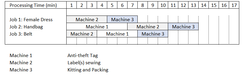
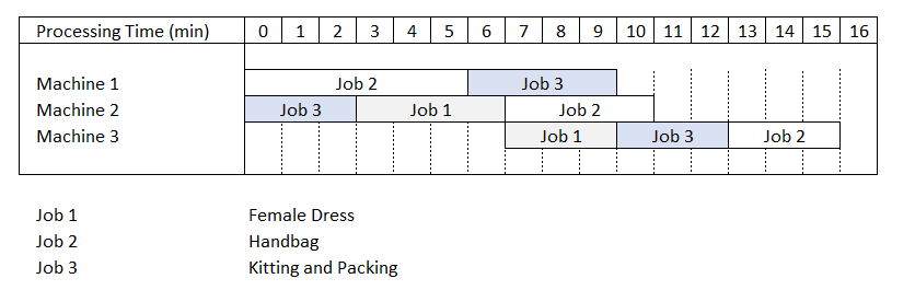
Our example with 3 jobs using 3 machines — (Image by Author)

For each job, we have defined the execution time (min) and the processing order of the machines in the table above.

For instance, Job 2 (Handbag) is starting with Anti-theft Tags placement using Machine 1 (6 min) followed by Labels Sewing using Machine 2 (4 min), to finally end with Kitting and Packing using Machine 3 (3 min).

The machines can only execute one job at a time.

Once started, the machine cannot be interrupted until the assigned job is complete.

Objective: minimise the makespan, i.e., the total time for completion of all jobs

i. The Naive Solution: 1 job cycle at a time

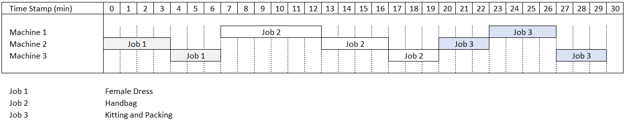
First Naive Approach — (Image by Author)

Results

Makespan: 30 min
Productivity: 2 sets/hour

Comments

This simple approach is the least productive.

Because jobs are processed sequentially, machines remain idle (unused) quite often.

Question: What would be the result if we performed jobs in parallel?

ii. Optimal Solution: The Job Shop Scheduling Problem using Google OR-Tools

OR-Tools is an open-source collection of tools from Google for combinatorial optimisation.

The objective is to identify the best solution from a large set of possible solutions.

I am a fan of this library that I have been using in several examples:

Design a Pathfinding Algorithm using Google AI to Improve Warehouse Productivity

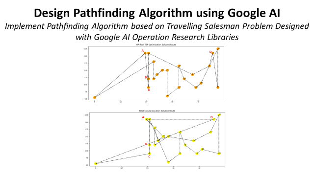
Optimise Workforce Planning using Linear Programming with Python

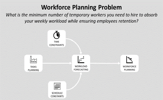
Let us use this library to find the optimal sequencing to reduce the makespan for this specific set of processes.

Optimisation of your Scheduling

Results: Optimised vs. Naive Solutions

Optimized Solution with Google OR-Tools — (Image by Author)

The two graphs above show the initial solution (Naive Solution: 1 job at a time) and the Optimised Solution (Parallel Tasking).

Results

Total Makespan: 16 min (-47%)
Productivity: 3.75 sets/hour (+85%)
Idle time per cycle: 18 min (-71.4%)

The results are satisfying

I will explain how to reach these results now.

If you prefer watching, a YouTube version is available

Build the optimisation model.

a. Initialise your model

b. Initialise variables and create sequences

c. Add Constraints and Set up the Solver

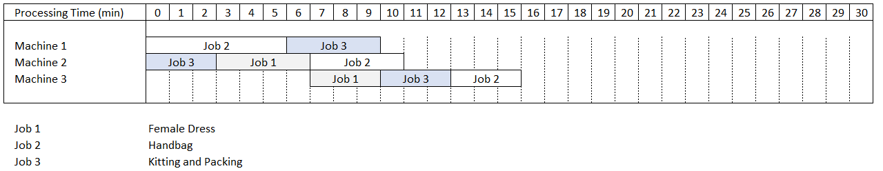
d. Solver Optimal Solution

Output
Optimal Schedule Length: 16
Machine 1: job_2_1 job_3_2 [0,6] [6,10]
Machine 2: job_3_1 job_1_1 job_2_2 [0,3] [3,7] [7,11]
Machine 3: job_1_2 job_3_3 job_2_3 [7,10] [10,13] [13,16]

Based on this output, we can draw the updated schedule:

Conclusion

💡

If you have any question, feel free to ask it here: Ask a Question

We increased productivity by 48% by implementing a smart scheduling solution that maximises the utilisation of our resources (Machines).

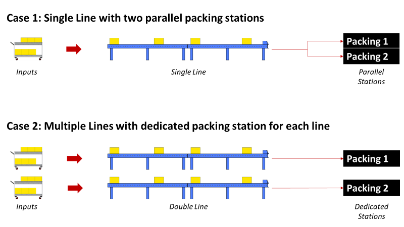
This solution was based on a simple scenario using a single line of assembly (1 Machine per Type).

Can we have higher productivity by changing the conditions?

Next Steps

In the chart below, I have highlighted the potential additional jobs we could add during the idle time:

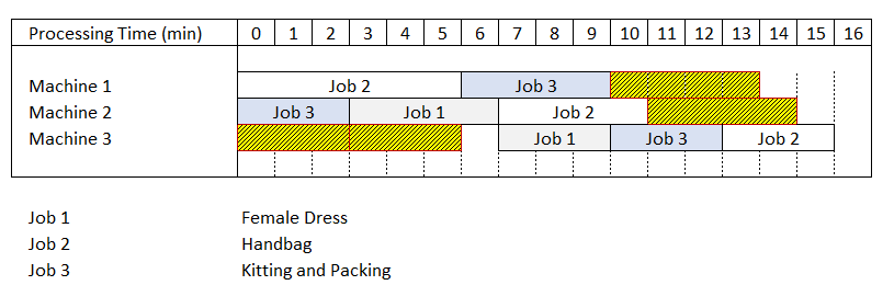
Optimized Solution with idle sequences (yellow) — (Image by Author)

Question: What would be the average productivity if we start Jobs of Cycle n+1 during these idle sequences of Cycle n?

Machine 1: 1 sequence of 4 min, which equals the time for Job 3
Machine 2: 1 sequence of 4 min, which equals the time for Job 1 and Job 2
Machine 3: 2 sequences of 4 min, which equals the time for Jobs 1,2 and 3

This raises additional questions related to the process design.

What happens if one job must wait for the previous job that encountered unpredictable issues?

This can be answered by using mathematical tools like the Queueing theory introduced in this article.

About Me

Let’s connect on LinkedIn and Twitter. I am a Supply Chain Engineer who is using data analytics to improve logistics operations and reduce costs.

If you’re looking for tailored consulting solutions to optimise your supply chain and meet sustainability goals, please contact me.