Improve Warehouse Productivity using Pathfinding Algorithm with Python
Implement Pathfinding Algorithm based on Travelling Salesman Problem Designed with Google AI Operation Research Libraries
Implement Pathfinding Algorithm based on Travelling Salesman Problem Designed with Google AI Operation Research Libraries
Pathfinding Algorithm for Picking Route Creation
In the first articles, we built a model to test several strategies of Orders Wave Creations to reduce the walking distance for picking by
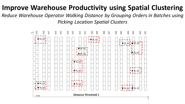
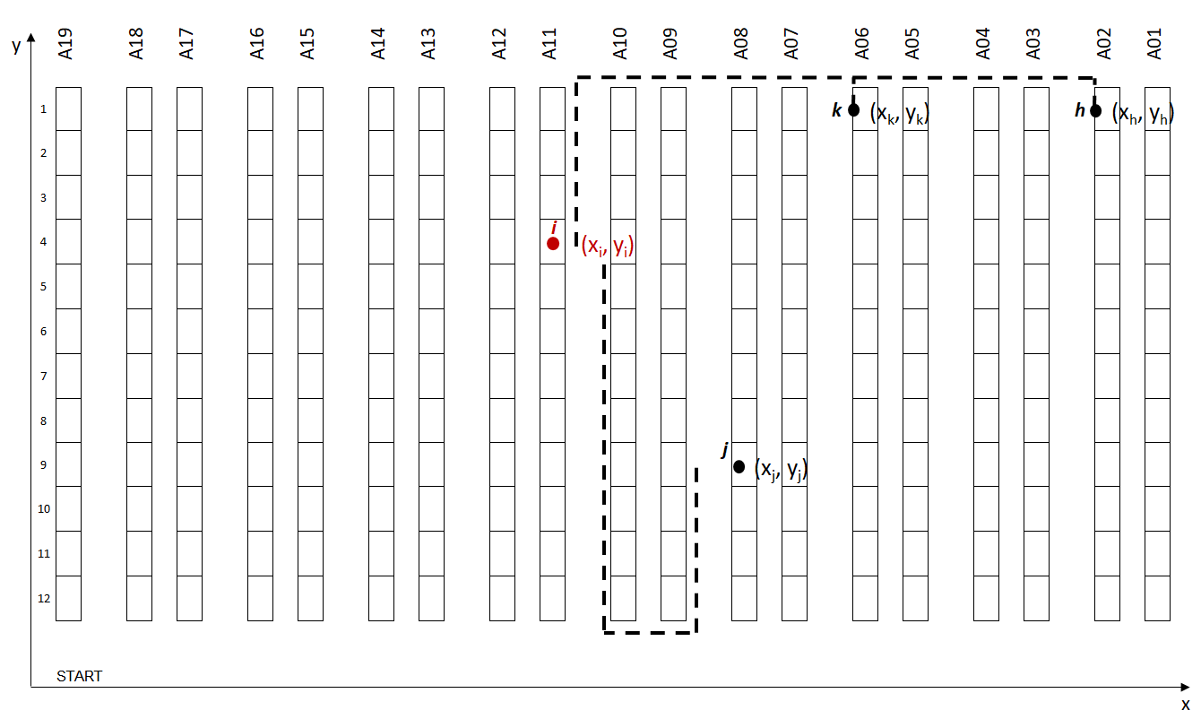
- Warehouse Mapping: link each order line with the associated picking location coordinate (x, y) in your warehouse
- Distance Calculation: a function calculating walking distance from two picking locations
- Picking Locations Clustering: functions grouping orders by waves using geographical (x, y) clusters to reduce the maximum distance between two locations in the same picking route
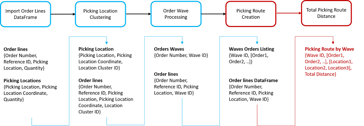
At this stage, we have orders grouped by waves to be picked together. For each wave, we have a list of picking locations that need to be covered by the Warehouse Picker.
The next target is to design a function to find a sequence of locations that will minimize walking distance.
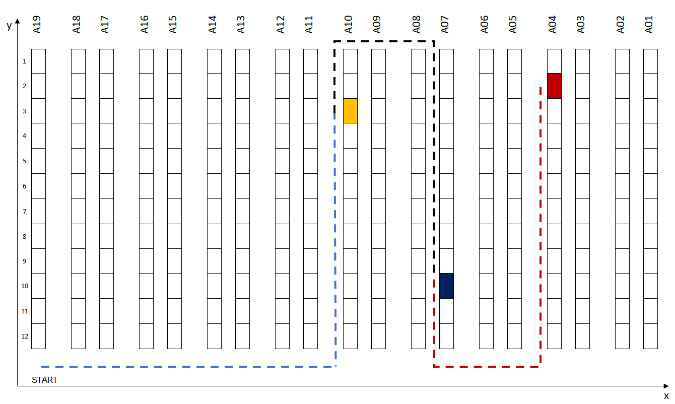
Initial Solution: Next Closest Location Strategy
In the first article, we presented an initial solution using the Next Closest Location Strategy.
This simple strategy does not require a high level of computational effort.
From a location j (xj, yj), this function will take as input a list of potential next locations [(xj, yj), (xk, yk), (xh, yh)].
The output will be the closest location, using a custom distance walking function, as the best candidate for the next location to cover.
Question: Is it the most optimal solution for Picking Route Creation ?
Travelling Salesman Problem Applied to Warehouse Picking Route Design
Objective: find the optimal algorithm for picking route creation using the Single Picker Routing Problem (SPRP) for a two-dimensional warehouse.
SPRP is a specific application of the general Traveling Salesman Problem (TSP) answering the question:
“Given a list of storage locations and the distances between each pair of locations, what is the shortest possible route that visits each storage location and returns to the depot ?”
Building a Travelling Salesman Model using Google AI’s OR-Tools
OR-Tools is an open-source collection of tools for combinatorial optimization. Out of a very large set of possible solutions, the objective is to find the best solution.

Here, we’re going to adapt their Travelling Salesman Problem use-case for our specific problem.
Adapt Google-OR Model
The only adaptation we need to do
Input Data
- List of picking locations coordinates:
List_Coord = [(xi, yi), (x2, y2), …, (x_n, y_n)] - Walking Distance Function
f: ((x_i, y_i), (x_j, y_j)) -> distance(i,j)
Code
In Google OR’s example, a dictionary is created with:
- Distance Matrix: [distance(i,j) for i in [1, n] for j in [1, n]]
- Number of Vehicles: 1 vehicle for our scenario
- Location for depot = start and end: start = end = List_Coord[0]
Simulation: OR-Tool Solution vs. Closest Next Location
The target is to estimate the impact on total walking distance if we use the TSP Optimized Solution of Google-OR vs. our initial Closest Next Location Solution.
We’re going to use the part 2 method to simulate scenarios
- Order lines: 20,000 Lines
- Distance Threshold: Maximum distance between two picking locations in each cluster (distance_threshold = 35 m)
- Orders per Wave: orders_number in [1, 9]
- 3 Methods for Clustering
Method 1: clustering is not applied
Method 2: clustering applied on single-line orders only;
Method 3: clustering on single-line orders and centroids of multi-line orders;
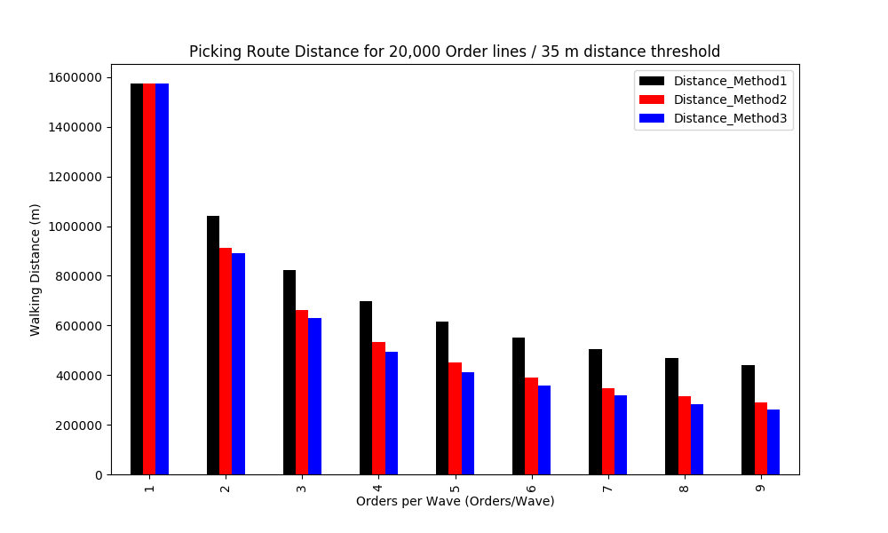
Best Performance
Method 3 for 9 orders/Wave with 83% reduction of Walking Distance
Question
How much can we reduce Walking Distance by applying TSP Optimized Solutions of Google-OR on top of this?
Code
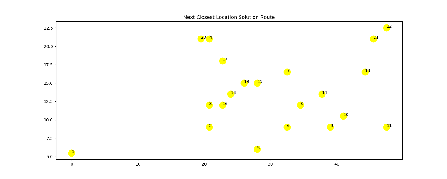
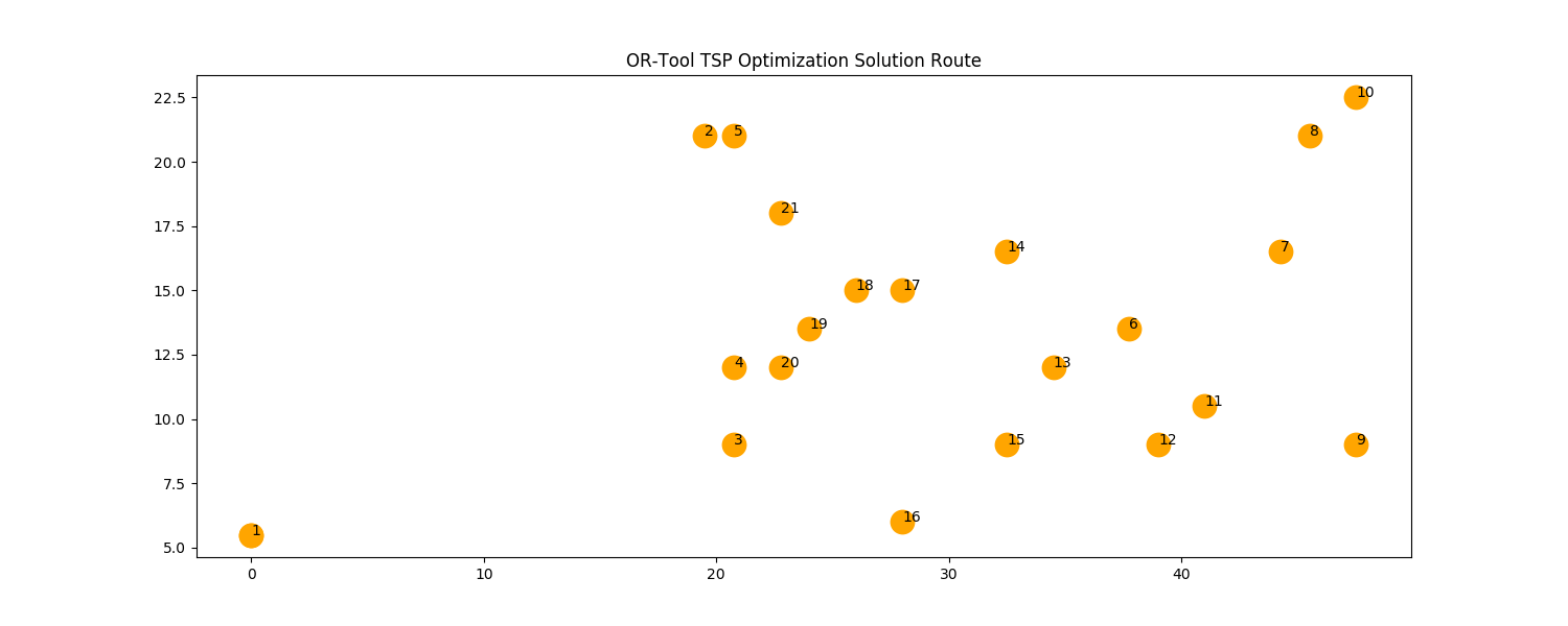
OR-Tool Solution vs. Closest Next Location
After running Waves using these three methods, we build picking routes using:
- Next Closest Location: distance_init
- TSP Optimized Solution of Google-OR: distance_or
- Distance Reduction (%): 100 * (distance_init-distance_or)/distance_init
Few Insights
- Orders per Wave: when orders number per wave OR-Tools is more impactful
- Methods: when clustering for Wave Processing is added OR-tools impact is lower
Best Scenario Result
Method 3 (Clustering for all orders) impact is -1.23 % of the total Walking Distance.
Learn more about Voice Picking Systems to implement this solution
Understand TSP Solution
For Method 3 (Clustering for all orders) OR-Tool TSP Solution reduces the total Walking Distance by 1.23 %.
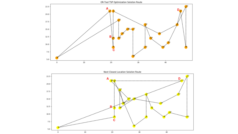
Let’s have a look at a specific example to understand.
Highest Gap: 60 m for 21 Picking Locations
A specific example is one picking wave with 21 Locations covered:
- OR-Tool TSP: Distance = 384 m
- Next Closest Location: Distance = 444 m
- Distance Reduction: 60 m
Limits of Next Closest Location (NCL) Algorithm
TSP Point 2 (Point A)
In this specific example, we can see the benefits of the TSP Optimization Solution for the second point (19.5, 21)
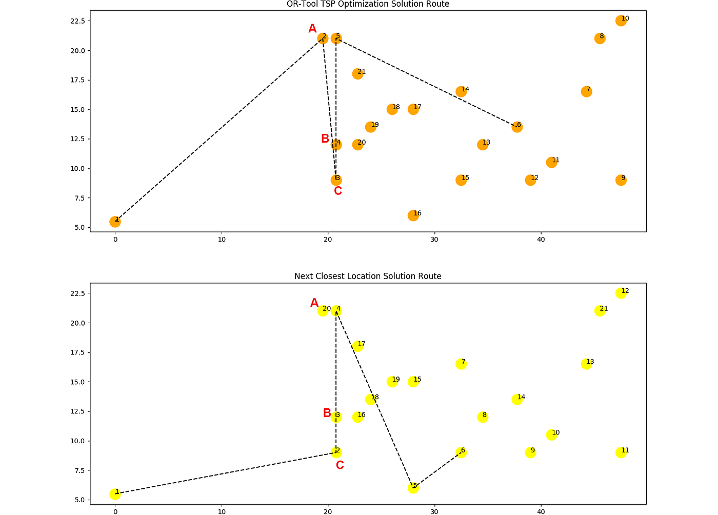
Starting at Point 1, the three closest points are {A, B, C}
- The closest point to Point 1 is A
- NCL Point is going directly to C, TSP starts from A
- TSP covers {A, B, C} in one time, while NCL only covers {B, C} and lets A for later
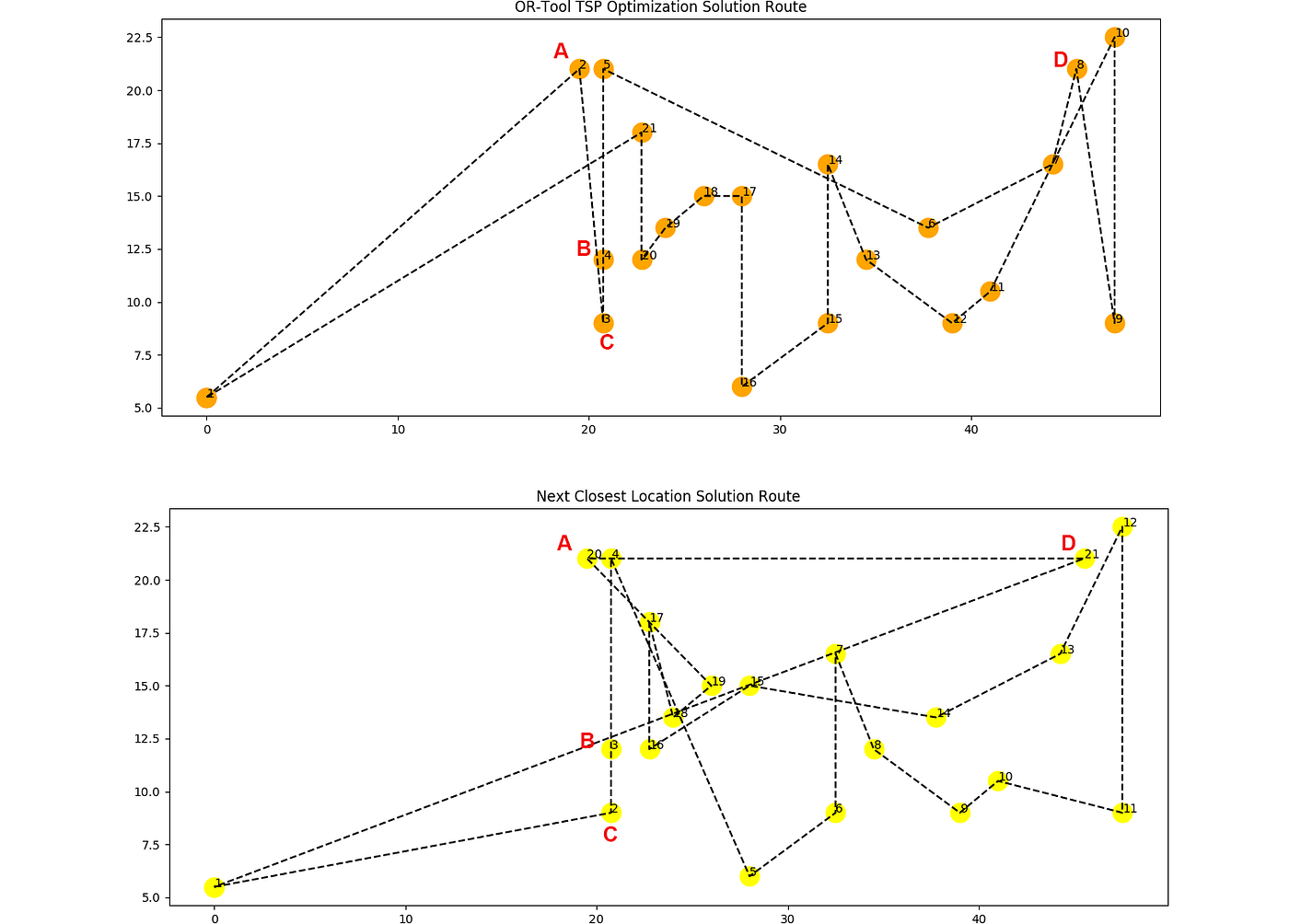
NCL Point 21
In the example above, after Point 20 (Point A), Warehouse Picker still needs to cover Point 21 (Point D) before going to Depot (Point 1).
This extra distance greatly impacts NCL efficiency for this Wave.
Conclusion
Applying the Travelling Salesman Problem Solution to the Picking Route Creation can reduce total Walking Distance and improve overall productivity.
Coupled with smart Order Wave Processing, it can optimize the sequence of picking for waves with a high number of picking locations by finding the shortest path to cover a maximum number of locations.
About Me
Let’s connect on Linkedin and Twitter, I am a Supply Chain Engineer that is using data analytics to improve logistics operations and reduce costs.
If you’re looking for tailored consulting solutions to optimize your supply chain and meet sustainability goals, please contact me.
References
[1] Google OR-Tools, Solving a TSP with OR-Tools, Link
[2] Samir Saci, Improve Warehouse Productivity using Order Batching with Python
 Samir Saci
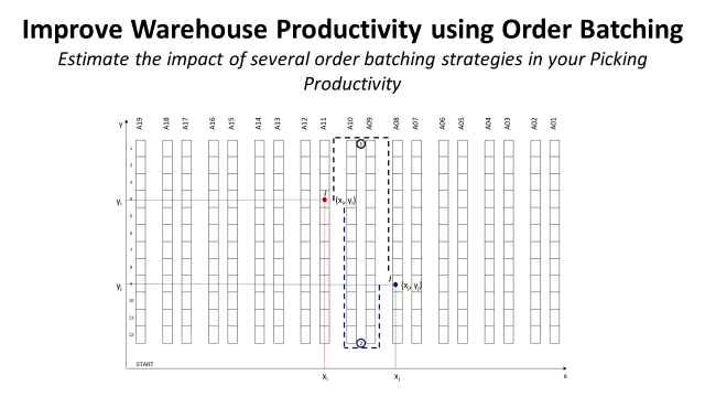
[3] Samir Saci, Improve Warehouse Productivity using Spatial Clustering for Order Batching with Python Scipy
Samir Saci