Machine Learning for Retail Sales Forecasting — Feature Engineering
Understand the impacts of additional features (stock-out, store closing date or cannibalisation) on an ML model for sales forecasting.
Based on feedback from the last Makridakis Forecasting Competitions, Machine Learning models can reduce forecasting error by up to 60% relative to benchmarks.
Their major advantage is the ability to incorporate external features that significantly affect sales variability.
For example, e-commerce cosmetics sales are driven by special events (e.g. promotions) and by features associated with how you advertise a reference on the website (e.g. first page, second page, …).
This process, called feature engineering, is based on analytical concepts and business insights to understand what could drive your sales.
In this article, we examine the impact of several features on the accuracy of a model using the M5 Forecasting competition dataset.
💌 New articles straight to your inbox for free: Newsletter
I. Introduction
1. Data set
2. Initial Solution using LGBM
3. Features Analysis
II. Experiment
1. Additional features
2. Results
III. Conclusion and next steps
Introduction
Data set
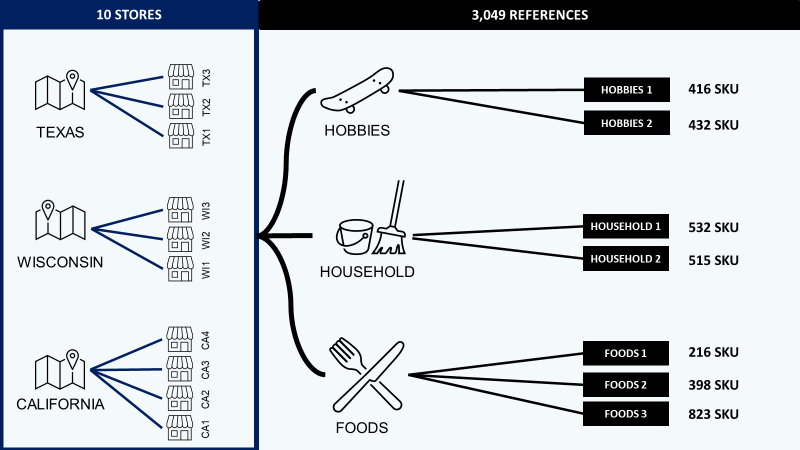
This analysis will be based on the M5 Forecasting dataset of Walmart store sales records.
- 1,913 days for the training set and 28 days for the evaluation set
- 10 stores in 3 states (USA)
- 3,049 unique in 10 stores
- 3 main categories and 7 departments (sub-categories)
The objective is to predict sales for all products in each store in the 28 days following the available dataset.
We will generate 30,490 forecasts for each day in the prediction horizon.
We’ll use the validation set to measure the performance of our model.
Initial Solution using LGBM
As a base model, we will use the solution introduced in a previous article.
In this notebook, you will find all the different steps to build a quite good model with a reasonable computing time:
- Import and processing of raw data
- Exploratory Data Analysis
- Features Engineering
i) Seasonality: week number, day, month, day of the week
ii) Pricing: the weekly price of an item in each store, special events
iii) Trends: sales lags (n-p days), average volume per {item, (item +store)}, …
iv) Categorical Variables encoding: item, store, department, category, state
- Model Training: 1 model LightGBM per store
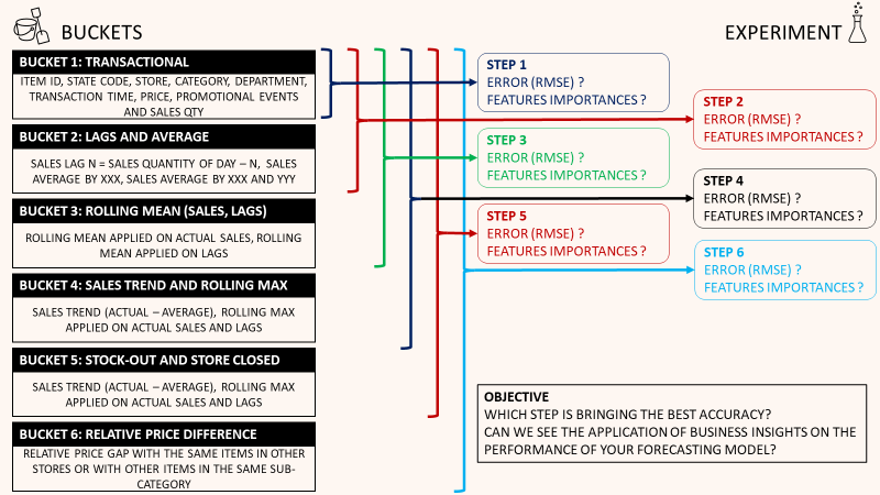
Features Engineering
To emphasise the impact of feature engineering, we will not change the model and will examine only which features we use.
Let us split the features used in this notebook into different buckets.
—
Bucket 1: Transactional Data
'id', 'item_id',
# Store, Category, Department
'dept_id', 'cat_id', 'store_id', 'state_id'
# Transaction time
'd', 'wm_yr_wk', 'weekday', 'wday', 'month', 'year'
# Sales Qty, price and promotional events
'sold', 'event_name_1', 'event_type_1', 'event_name_2', 'event_type_2', 'sell_price'
events and sell_price
Capture the impact on sales of a special event on an item of selling price XXX.
What could be the impact of a special event with a 20% reduction on sales of baby formula the second week of the month?
Open Question
What would be the impact on the accuracy if we do one-hot encoding for the categorical features?
—
Bucket 2: Sales Lags and Average
'sold_lag_1', 'sold_lag_2', 'sold_lag_3', 'sold_lag_7', 'sold_lag_14', 'sold_lag_28'
# Sales average by
'item_sold_avg', 'state_sold_avg','store_sold_avg', 'cat_sold_avg', 'dept_sold_avg'
# Sales by XXX and YYYY
'cat_dept_sold_avg', 'store_item_sold_avg', 'cat_item_sold_avg','dept_item_sold_avg', 'state_store_sold_avg','state_store_cat_sold_avg', 'store_cat_dept_sold_avg'
lags
Measure the week-on-week or month-on-month (7 days, 28 days) similarities to capture the periodicity of sales due to people shopping at these frequencies.
Do you have relatives going to the hypermarket every Saturday to shop for the whole week?
Experiment
Additional features
Based on business insights, we will add features to help our model capture all key factors affecting customer demand.
—
Bucket 3: Rolling Mean and Rolling Mean applied on lag
'rolling_sold_mean', 'rolling_sold_mean_3', 'rolling_sold_mean_7','rolling_sold_mean_14', 'rolling_sold_mean_21', 'rolling_sold_mean_28'
# Rolling mean on lag sales
'rolling_lag_7_win_7', 'rolling_lag_7_win_28', 'rolling_lag_28_win_7', 'rolling_lag_28_win_28'
rolling_sold_mean_n
Measure the average sales of the last n days.
The rolling mean is sometimes used as a benchmark for statistical forecasting.
Code
rolling_lag_n_win_p
Measure the average sales of a p days windows ending n days ago.
Code
BUSINESS INSIGHTS
Sunglasses seasonality
If the rolling mean of the last 7 days is 35% higher than the average sales of the week before, that means you have started the summer season.
—
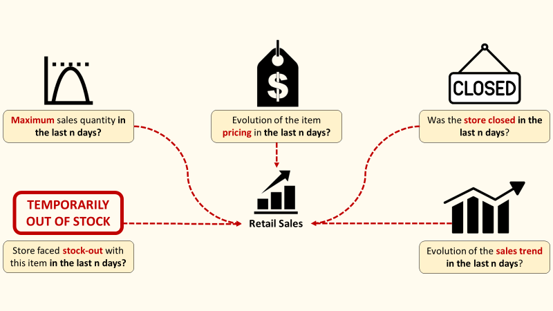
Bucket 4: Sales Trend and Rolling Maximum
'selling_trend', 'item_selling_trend'
# Rolling max
'rolling_sold_max', 'rolling_sold_max_1', 'rolling_sold_max_2', 'rolling_sold_max_7', 'rolling_sold_max_14', 'rolling_sold_max_21','rolling_sold_max_28'
Selling trend
Measure the gap between the daily sales and the average.
Code
Rolling max
What is the maximum sales in the last the n days?
Code
Spoiler: this feature will have an important impact on your accuracy.
—
Bucket 5: Stock-Out and Store Closed
'stock_out_id'
# Store closed
'store_closed'
stock-out
Explain that you have zero sales because of stock availability issues.
Code
—
Bucket 6: Price Relative to the same item in other stores or other items in the sub-category
'delta_price_all_rel'
# Relative delta price with the previous week
'delta_price_weekn-1'
# Relative delta price with the other items of the sub-category
'delta_price_cat_rel'
delta_price_weekn-1
Capture the price evolution week by week.
BUSINESS INSIGHTS
Promotions for Slow Movers
To reduce inventory and purge slow-moving items, stores may implement aggressive pricing to boost sales.
delta_price_all_rel: Sales Cannibalization at store level
Several stores competing for sales of the same item because of price difference.
delta_price_cat_rel: Sales Cannibalization at sub-category level
Several items of the same sub-category competing for sales.
Code
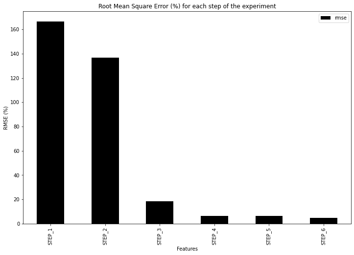
Results
After running a loop of training with the six different buckets (using the same hyperparameter with the Kaggle notebook), we have the following results:
—
STEP 1 to STEP 2: -29% RMSE Error
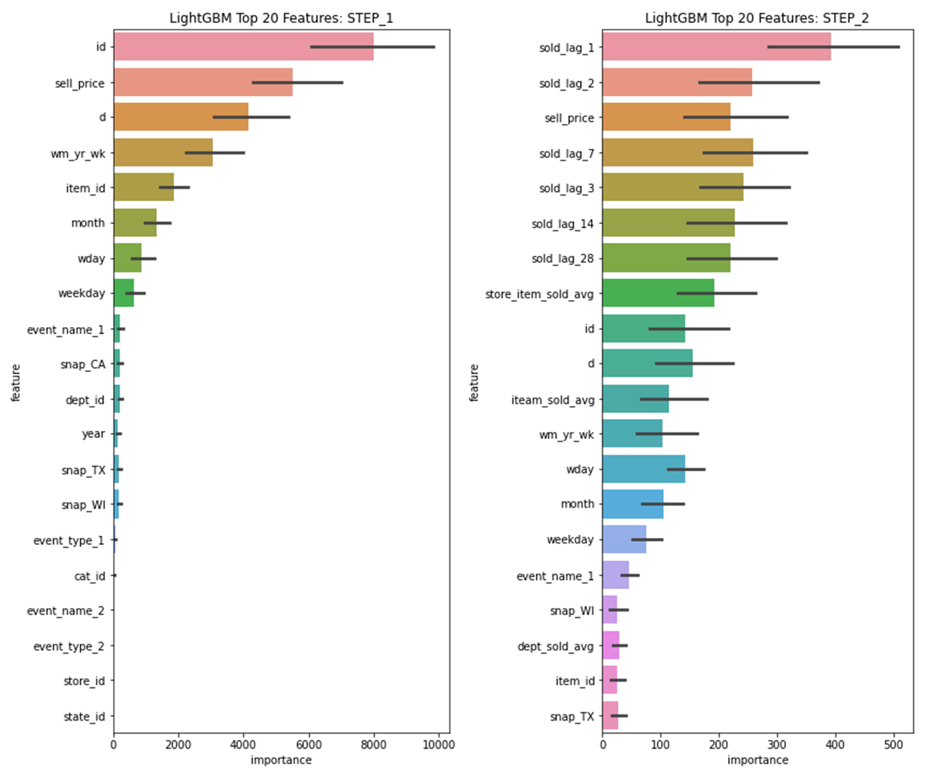
Sales lags are positively impacting the accuracy of your model:
BUSINESS INSIGHTS
Your sales today are highly impacted by the sales of previous days.
—
STEP 2 to STEP 3: -118% RMSE Error
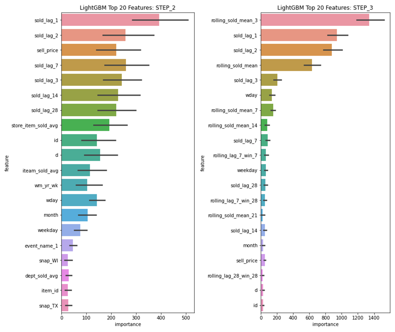
BUSINESS INSIGHTS
The top 3 features are all related to sales over the last 3 days.
Question
Based on this insight, what could be the performance of a model like Exponential Smoothing who is taking a ponderate sum of the previous sales to compute the forecasts.
—
STEP 3 to STEP 4: -12% RMSE Error
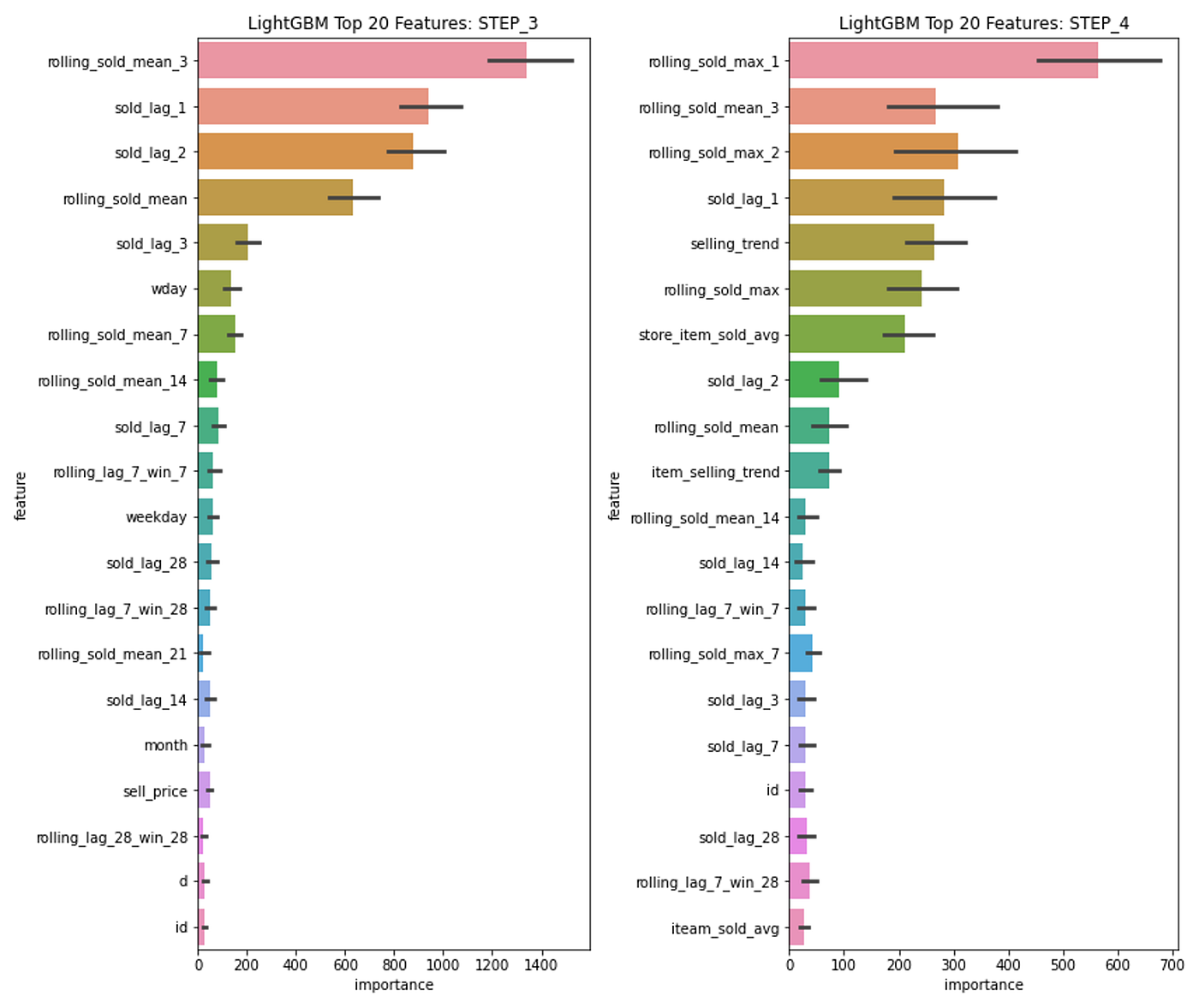
Rolling max features are taking the lead at the top of the features.
—
STEP 4 to STEP 5: -0.1% RMSE Error
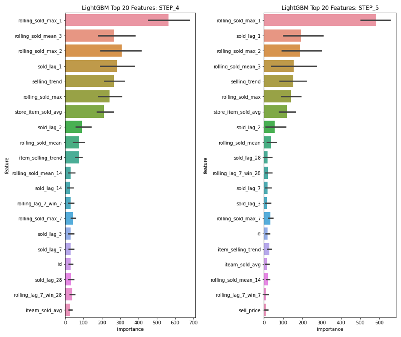
BAM!
I am devastated to see that the potential main added value of this article, showing the impact of stock-out or store closing, has a limited impact on the accuracy of the model.
—
STEP 5 to STEP 6: -1.75% RMSE Error
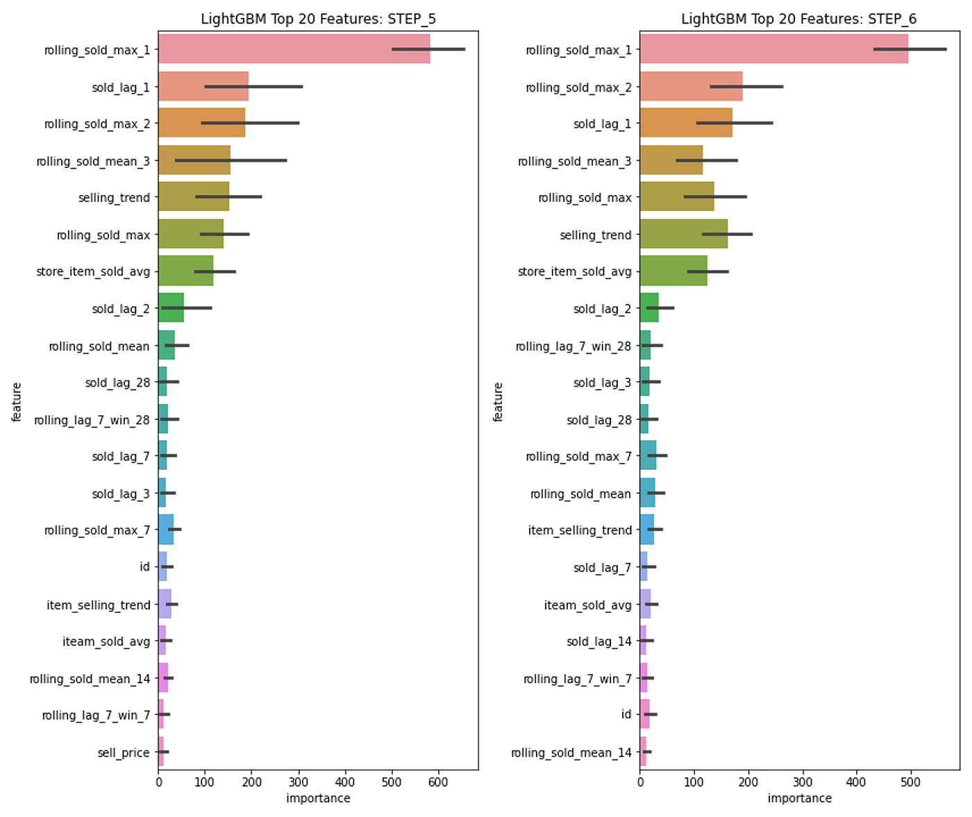
The model's accuracy is slightly higher, but none of the added features appear among the top 20.
Implement this on your machine!
Conclusion and next steps
Understand the results
The model accuracy results are quite satisfactory.
However, there remains frustration at the lack of a correlation between certain newly added features and model performance.
If these business insights are not improving your forecasts, we need to understand why.
What's next?
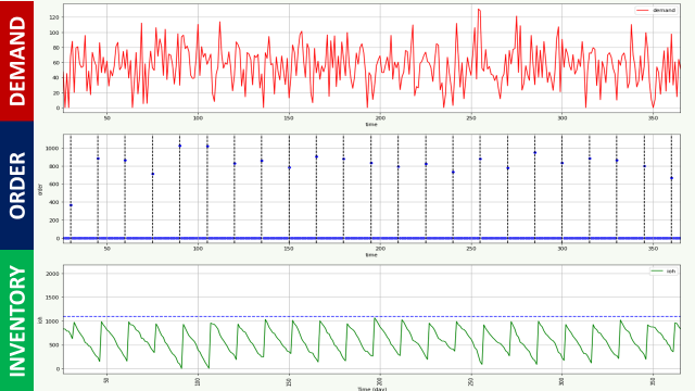
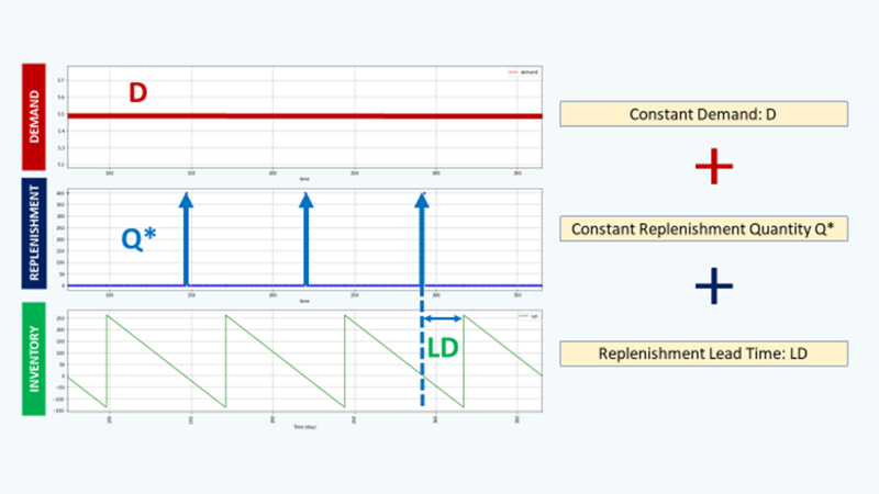
Implement Inventory Management Rules
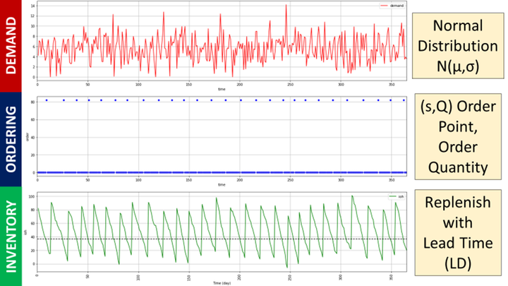
Now that you have your forecasting model, you need to implement an inventory management rule to manage store replenishment.
You can start with this article to understand the basics of inventory management rules using a simple example that assumes deterministic demand:
This article includes a complete video tutorial in which you will build the entire modelisation in a Jupyter Notebook.
It's a great start to learn inventory policies.
Have you heard about Green Inventory Management?
This is a sustainable approach of store replenishment focusing on optimising delivery frequencies to reduce the environmental and costs of distribution.
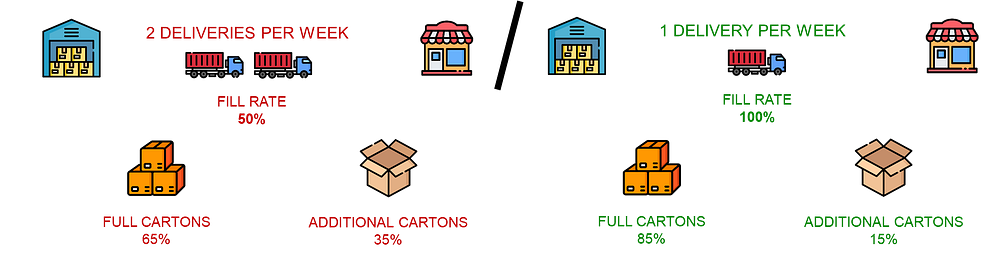
The idea is to find the optimal frequency that will:
- Minimise carton and film usage in the warehouse
- Maximise truck filling rate
- Minimise CO2 emissions
I have experiement the usage of AI agents to do that using a local MCP server connected to my Claude Desktop.
More details in this video,
About Me
Let’s connect on LinkedIn and Twitter. I am a Supply Chain Engineer who is using data analytics to improve logistics operations and reduce costs.
If you’re looking for tailored consulting solutions to optimise your supply chain and meet sustainability goals, feel free to contact me.