Machine Learning for Retail Demand Forecasting

Comparative study of Demand Forecasting Methods for a Retail Store (XGBoost Model vs. Rolling Mean)

💌 New articles straight to your inbox for free: Newsletter

Demand Planning Optimisation Problem Statement

For most retailers, demand planning systems take a fixed, rule-based approach to forecasting and replenishment order management.

Such an approach works well enough for stable, predictable product categories, but can show its limits in Inventory and Replenishment Optimisation.

This can reduce operational costs by:

• Inventory: matching store inventory with actual needs to reduce storage space needed (Rental Costs)
• Replenishment: minimise the number of replenishments between the warehouse and stores (Warehousing & Transportation Costs)

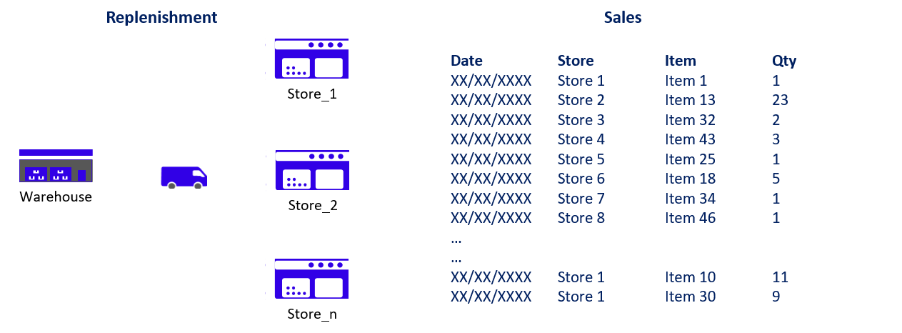
Example: Retailer with 50 Stores

For this study, we’ll take a dataset from the Kaggle challenge: Store Item Demand Forecasting Challenge.

Scope

• Transactions from 2013–01–01 to 2017–12–31
• 913,000 Sales Transactions
• 50 unique SKU
• 10 Stores

XGBoost for Sales Forecasting

The initial dataset was used in a Kaggle challenge, in which teams competed to design the best model to predict sales.

The first objective is to develop a predictive model using XGBoost.

This model will be used to optimize our replenishment strategy ensuring efficient inventory management and reducing the number of deliveries from your Warehouse.

Add Date Features

Daily, Monthly Average for Train

Add Daily, Monthly Averages to Test and Rolling Averages

Heat Map to check correlation

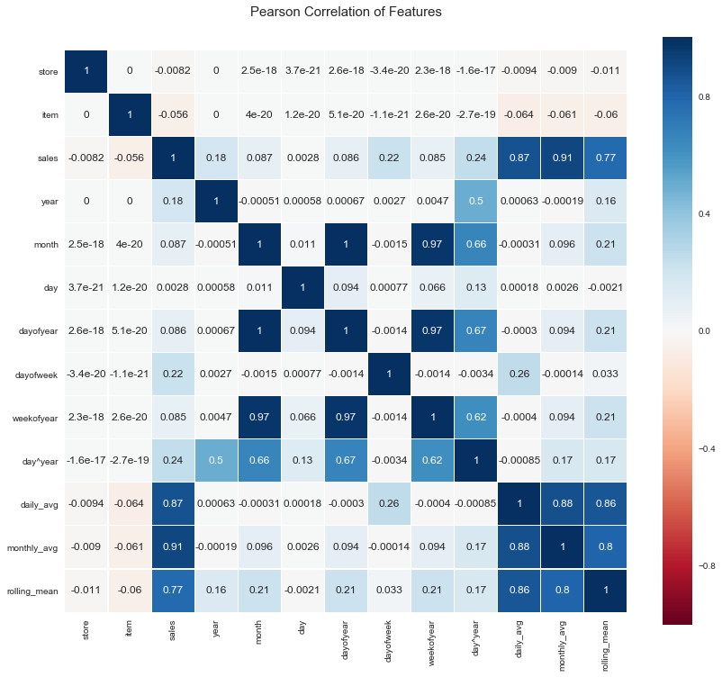
We will retain the monthly average, as it has the highest correlation with sales.

Remove other features that are highly correlated with each other.

Clean features, Training/Test Split and Run model

Results Prediction Model

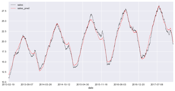
Based on this prediction model, we’ll build a simulation model to improve demand planning for store replenishment.

DataFrame Features

• date: Transaction date
• item: SKU Number
• store: Store Number
• sales: Actual value of sales transaction
• sales_prd: XGBoost prediction
• error_forecast: sales_prd — sales
• repln: boolean value for replenishment days (if the day is in [‘Monday’, Wednesday’, ‘Friday’, ‘Sunday’] return True)

Demand Planning: XGBoost vs. Rolling Mean

Demand Planning using Rolling Mean

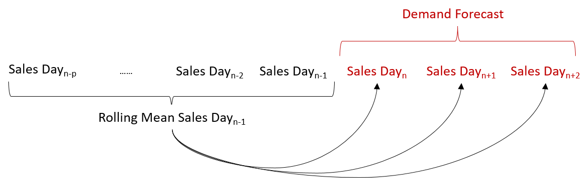
The first method to forecast demand is the rolling mean of previous sales. At the end of Day n-1, you need to forecast demand for Day n, Day n+1, and Day n+2.

1. Calculate the average sales quantity of the last p days: Rolling Mean (Day n-1, …, Day n-p)
2. Apply this mean to the sales forecast of Day n, Day n+1, Day n+2
3. Forecast Demand = Forecast_Day_n + Forecast_Day_(n+1) + Forecast_Day_(n+2)

2. XGBoost vs. Rolling Mean

With our XGBoost model available, we now have two demand-planning methods: the Rolling Mean Method.

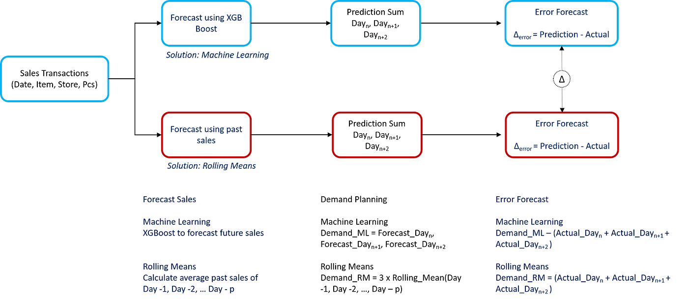
Let us try to compare the results of these two methods on forecast accuracy:

1. Prepare Replenishment at Day n-1
   We need to forecast replenishment quantity for Day n, Day n +1, Day n+2
2. XGB prediction gives us a demand forecast
   Demand_XGB = Forecast_Day(n) + Forecast_Day(n+1) + Forecast_Day(n+2)
3. Rolling Mean Method gives us a
   Demand_RM = 3 x Rolling_Mean(Day(n-1), Day(n-2), .. Day(n-p))
4. Actual Demand
   Demand_Actual = Actual_Day(n) + Actual_Day(n+1) + Actual_Day(n+2)
5. Forecast Error
   Error_RM = (Demand_RM — Demand_Actual)
   Error_XGB = (Demand_XGB— Demand_Actual)

With these indicators on hand, we can compare the different approaches.

a. Parameter tuning: Rolling Mean for p days

Before comparing the Rolling Mean results with XGBoost, we should determine the optimal value of p to achieve the best performance.

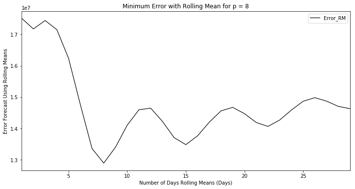
Results: -35% of error in forecast for (p = 8) vs. (p = 1)

Thus, based on the sales transactions profile, we caachieve optimalst demand planning performance by forecastinnext-day's saley using the average of the last 8 days.

b. XGBoost vs. Rolling Mean: p = 8 days

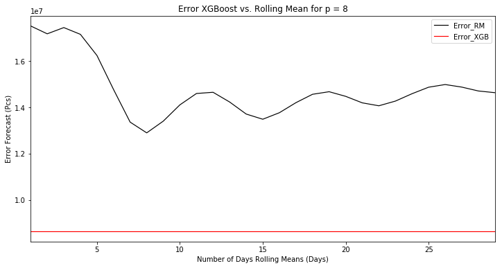
Results: -32% of error in the forecast by using XGBoost vs. Rolling Mean

Conclusion

Using the Rolling Mean method for demand forecasting, we could reduce forecast error by 35% and find the best parameter p days.

However, we could get even better performance by replacing the rolling mean with an XGBoost forecast to predict day n, day n+1 and day n+2 demand, reducing error by 32%.

Improve the model

I have been working on an improved version of the model presented in this article.

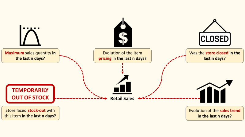
The goal is to assess the impact of adding business features (e.g., price changes, sales trends, store closures) on the model's accuracy.

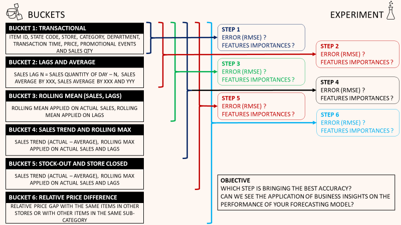
We use the model we are building here as the core and improve it with additional business insights.

For more details,

Machine Learning for Retail Sales Forecasting - Features

Understand the impacts of additional features (stock-out, store closing date or cannibalisation) on an ML model for sales forecasting.

Samir SaciSamir Saci

Next steps

• Inventory level: using XGBoost forecast to match inventory quantity with demand
• Order Frequency: Reduce order frequency using our forecasting model to match order quantity with demand

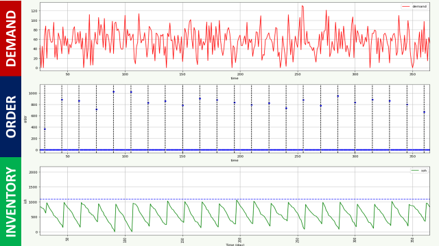
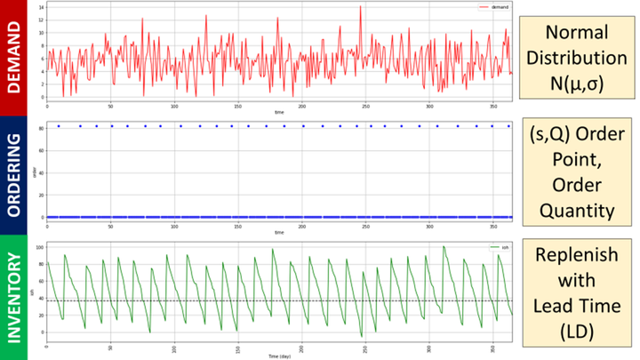
There are many inventory management rules that could be implemented based on these forecasts.

Never heard of inventory management rules? I have something for you.

In this complete tutorial, we learn the basics of inventory management by building replenishment rules for a deterministic demand.

More in the video,

About Me

Let’s connect on LinkedIn and Twitter. I am a Supply Chain Engineer who uses data analytics to improve logistics operations and reduce costs.

If you’re looking for tailored consulting solutions to optimise your supply chain and meet sustainability goals, feel free to contact me.