Inventory Management for Retail — Deterministic Demand

Build a simple model to simulate the impact of several replenishment rules (Basic, EOQ) on the inventory costs and ordering costs

Article originally published on Medium.

For most retailers, inventory management systems take a fixed, rule-based approach to forecast and replenishment order management.

Considering the distribution of the demand, the objective is to build a replenishment policy that will minimize your ordering, holding and shortage costs.

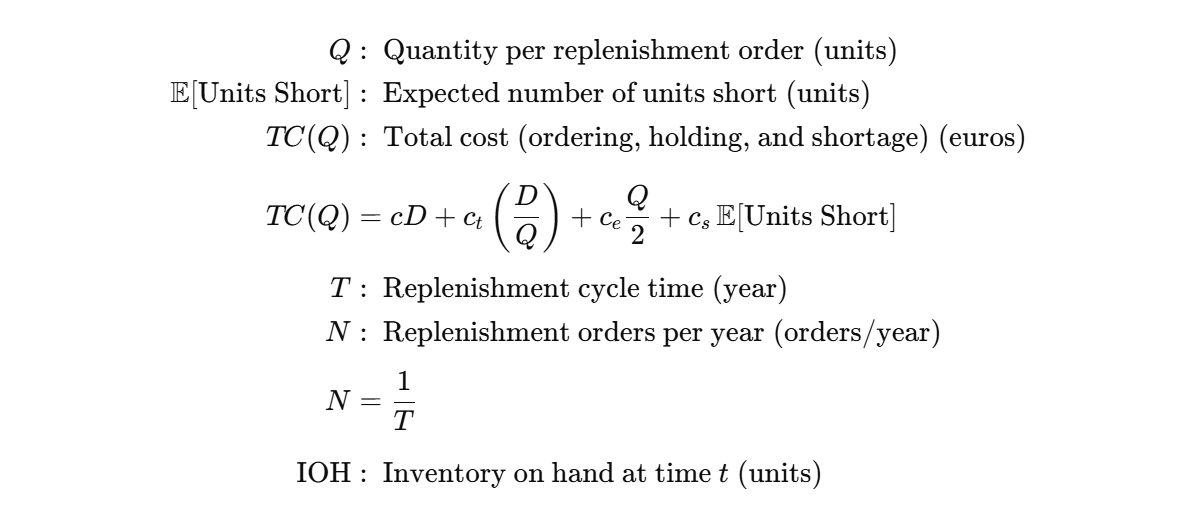
• Ordering Costs: fixed cost to place an order due to administrative costs, system maintenance or manufacturing costs in (Euros/Order)
• Holding Costs: all the costs required to hold your inventory (storage, insurance, and capital costs) in (Euros/unit x time)
• Shortage/Stock-out Costs: the costs of not having enough inventory to meet the customer demand (Lost Sales, Penalty) in (Euros/Unit)

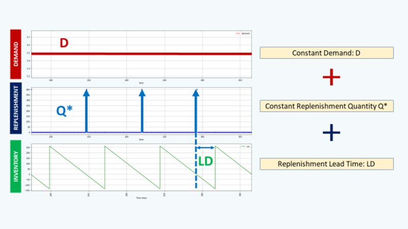
In this article, we will present a simple methodology using a discrete simulation model built with Python to test several inventory management rules based on assuming:

• Deterministic Constant Demand: D (Units/Year)
• Lead Time between ordering and replenishment (Days)
• Cost of shortage and storage (Euros/Unit)

💌 New articles straight in your inbox for free: Newsletter

I. Scenario

Problem Statement

As an Inventory Manager of a mid-size retail chain, you are in charge of setting the replenishment quantity in the ERP.

Based on the feedback of the store manager, you start to doubt that the replenishment rules of the ERP are the most optimal especially for the fast runners because your stores are facing lost sales due to stock-outs.

For each SKU, you would like to build a simple simulation model to test several inventory rules and estimate the impact on:

• Total Costs: how much does it cost to receive, store and sell this product?
• Shortages: what is the % of lost sales due to stock-out?

In this article, we will build this model for,

To simplify the comprehension, let’s introduce some notations

Objective

In this article, we will

1. Visualize the current rule used by the store's manager
2. Calculate the Economic Order Quantity and simulate the impact
3. Visualize the impact of lead time between ordering and receiving
4. Real-Time Visualization of COGS for each rule

II. Build Model

Economic Order Quantity (EOQ)

The theory behind the Economic Order Quantity (EOQ) that is used by many Inventory Optimization models is to find the optimal order quantity Q* that will be the best compromise between ordering costs and holding costs.

• A low order quantity will give you high ordering costs (increase the number of replenishment orders: D/Q) but will reduce your holding cost (reduce the average inventory level: (Q/2))
• The inverse for a high order quantity

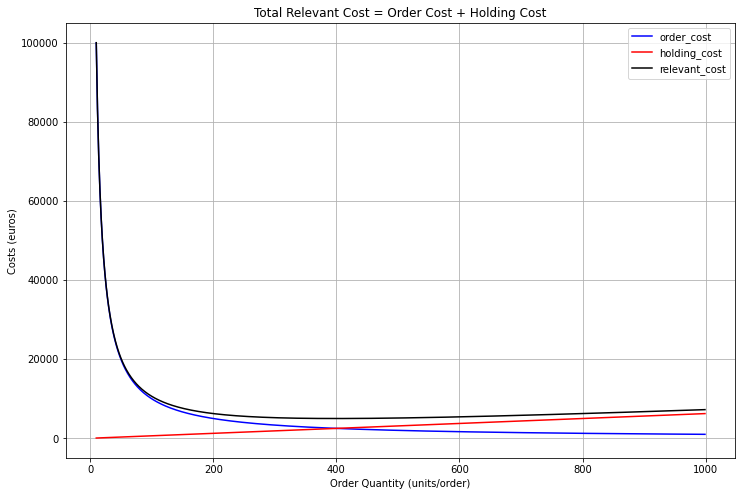
Comments

In the chart above we can see that the Total Relevant Cost (TRC) (total cost without the purchase cost cD) is minimum for Q*=400 units/order.

TRC(Q*) = 5,000 Euros

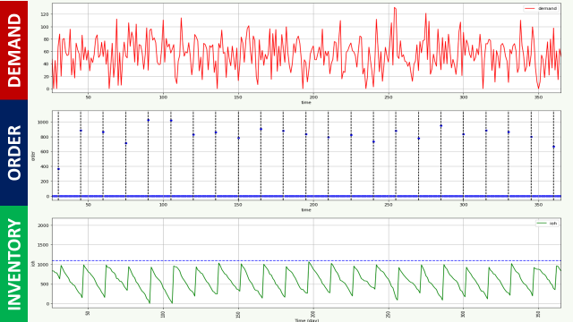
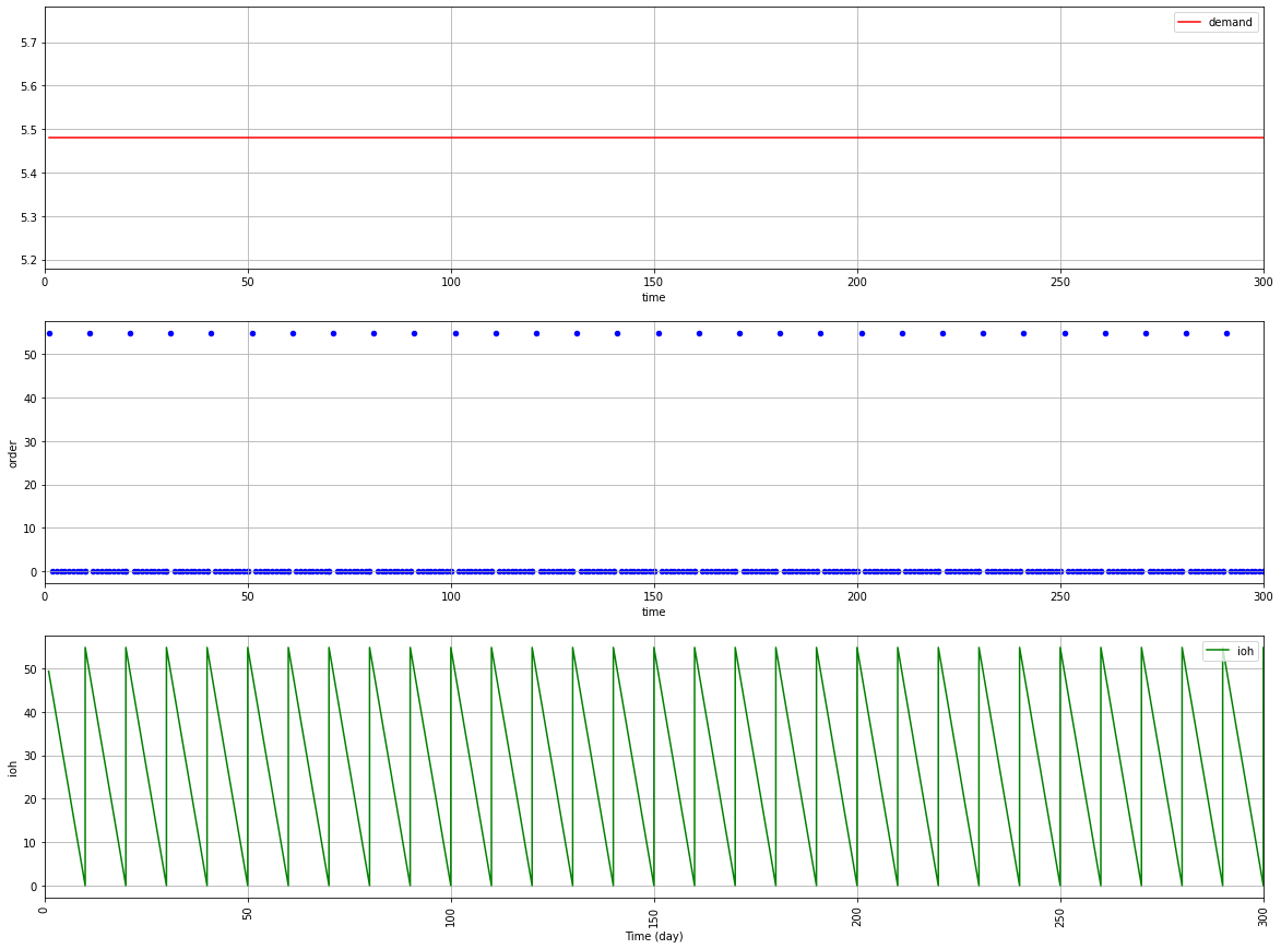
1. Visualize the current rule

The current rule is to order every 10 days the exact quantity needed to absorb the demand for 10 days.

This quantity is way lower than Q*, we can easily understand that the TRC will be way higher than its optimal value:

TRC(10) = 100,062 Euros

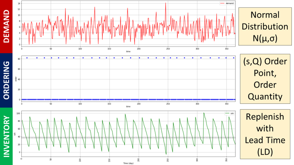
To understand why let’s simulate the rule for a range of 365 days:

Comments
Very short replenishment cycles that multiply the number of replenishment orders.

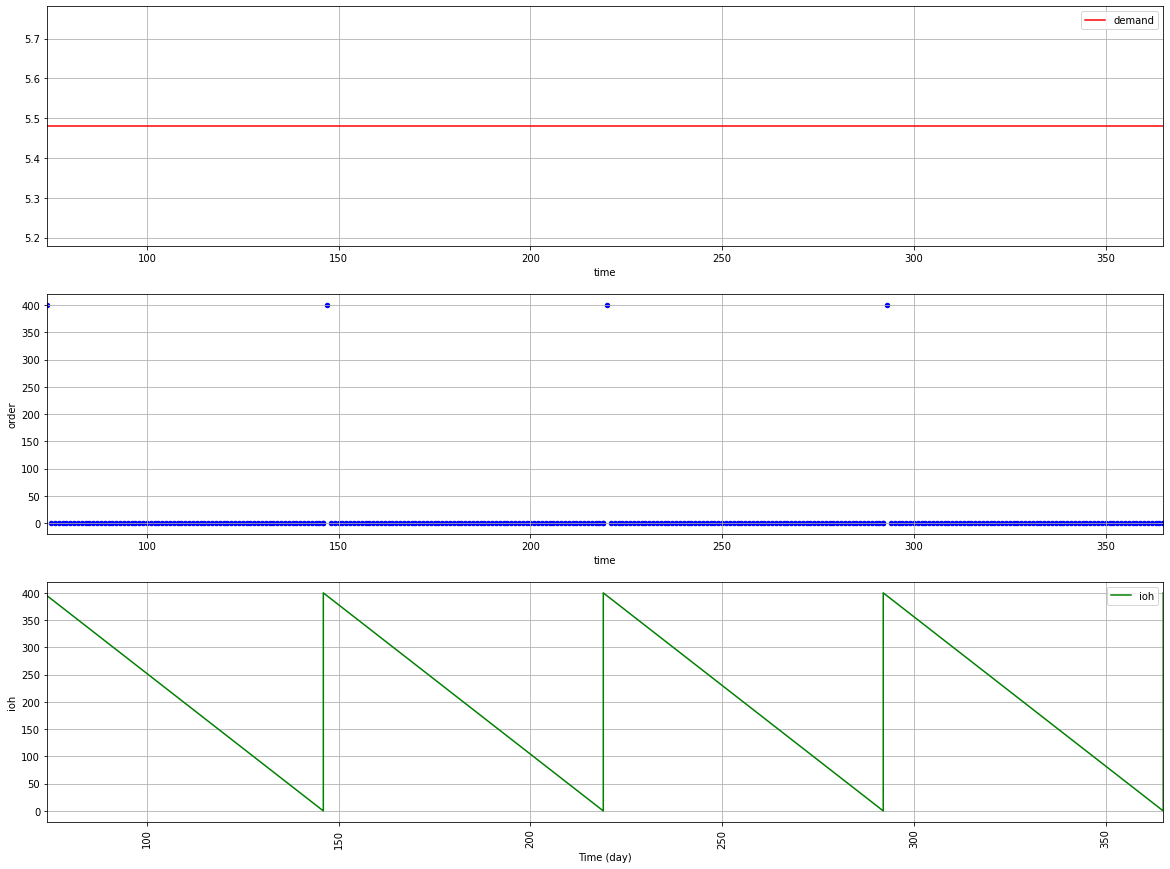
2. Economic Order Quantity: Q = Q*

For each replenishment cycle, you order Q* = 400 orders and you reorder when the inventory level is zero.

Comments
Longer replenishment cycles that reduce the number of orders by 7 times => lower TRC

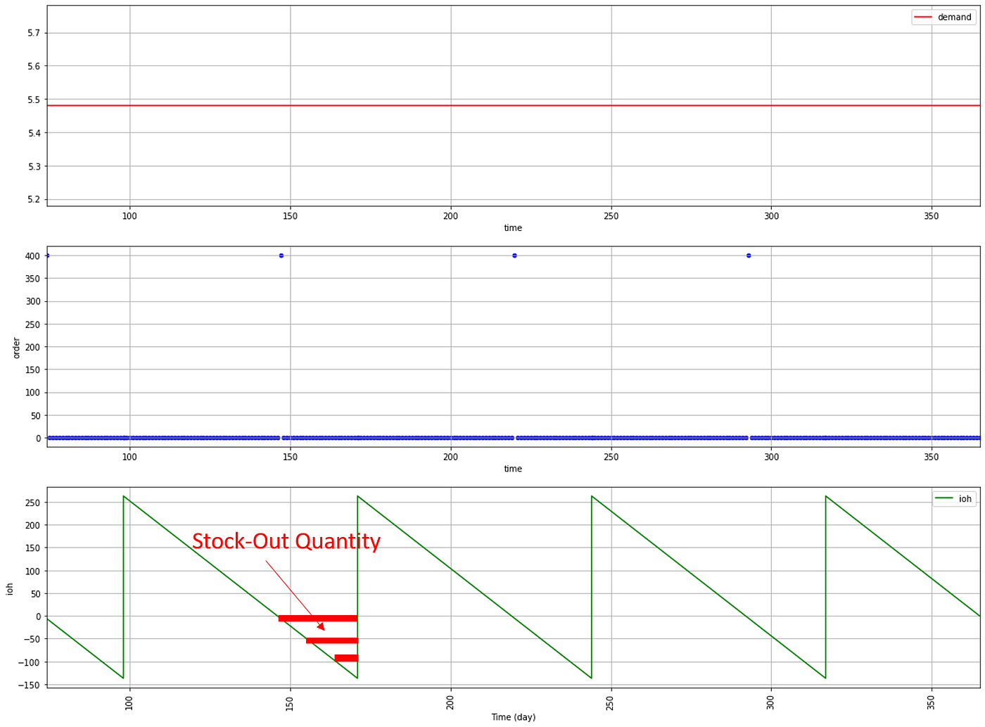
3. Include replenishment lead time

What would be the stock-out level if we have a replenishment lead time LD = N Days?

Comments
With 25 days lead time between ordering and receiving we reach 140 units of stock-out quantity per replenishment cycle.

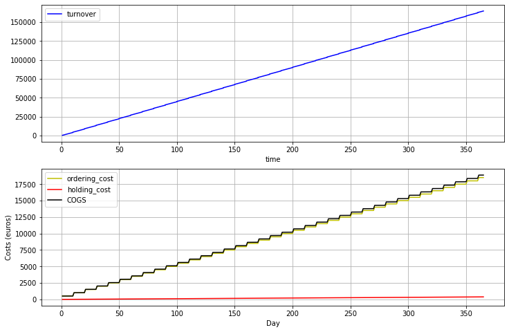
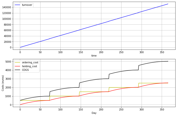
4. Real-Time visualization of Cost of Goods Sold (COGS)

If you want to convince your commercial team and the store managers; you need to speak their languages.

You can prepare a simple visualization of the potential turnover with the COGS (here we’ll exclude purchase costs COGS = TRC) to understand the impacts throughout the year.

Initial Rule

Comments
COGS is mainly driven by the ordering costs because of the high frequency of reordering due to the low replenishment quantity.

EOQ Rule

Comments
We see here that the Economic Order Quantity is providing a compromise between ordering costs and holding costs that drastically reduce the total COGS.

III. Conclusion & Next Steps

Conclusion

This simple modelisation was the occasion to design a basic simulation model that shows the impact of customer demand and inventory rules on key performance metrics.

It gives you visibility on your ordering frequency, inventory level and the impacts of lead times in your supply chain.

Next Steps

The initial assumption of constant deterministic demand is very optimistic. In the next article, we’ll study the impact of the variability of the demand on the total relevant costs and the lost sales.

About Me

Let’s connect on Linkedin and Twitter, I am a Supply Chain Engineer that is using data analytics to improve logistics operations and reduce costs.

References

[1] Supply Chain Science, Wallace J. Hopp