The master production schedule is the main communication tool between the commercial team and production.

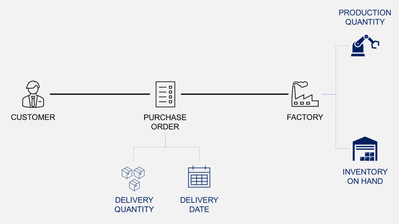
Your customers send purchase orders with specific quantities to be delivered at a certain time.

Production planning is used to minimise the total cost of production by balancing between minimal inventory and maximum quantity produced per setup.

In this article, we will implement optimal production planning using the Wagner-Whitin method with Python.

If you prefer to watch, have a look at the video version of this article

Problem Statement

Scenario

You are a production planning manager in a small factory producing radio equipment that serves local and international markets.

Customers send Purchase Orders (PO) to your commercial team with quantities and expected delivery dates.

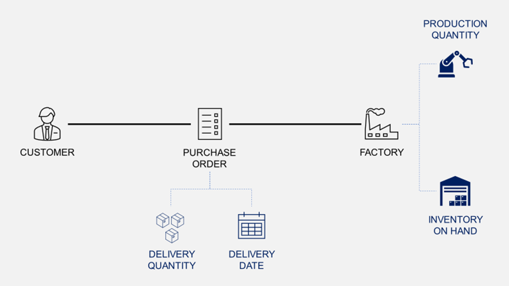
Your role is to schedule production to deliver on time with a minimum total cost of production that includes

• Setup Costs: fixed costs you have each time you set up a production line
• Production Costs: variable costs per unit produced
• Holding Costs: cost of storage per unit per time

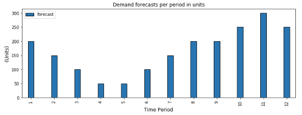
In our example, the customer ordered products for the next 12 months

Setup vs. Inventory Costs

The main challenges for you are

• Reducing the average inventory on hand to minimise the storage costs
• Minimise the number of production setups

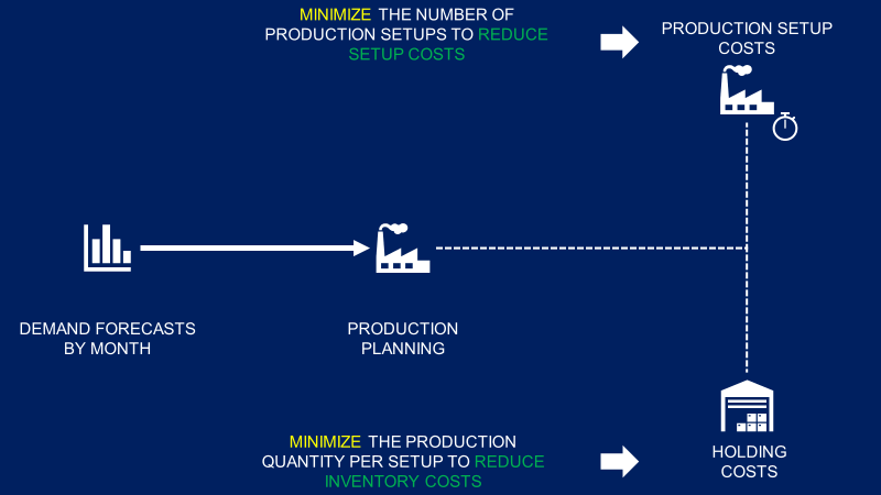
However, these two constraints are antagonistic. Therefore, it is difficult for you to find an intuitive way to build an optimal plan.

Example 1: Minimise Inventory

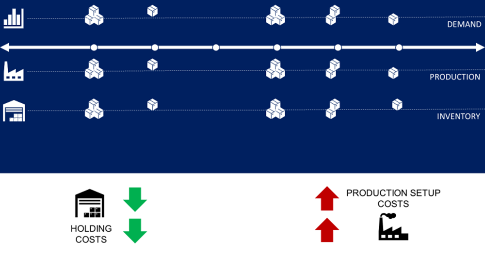
In this example, you produce the exact demand quantity each month

• Pros: no excess inventory
• Cons: You get production set up for each month with a positive demand

Example 2: Minimise the number of production setups

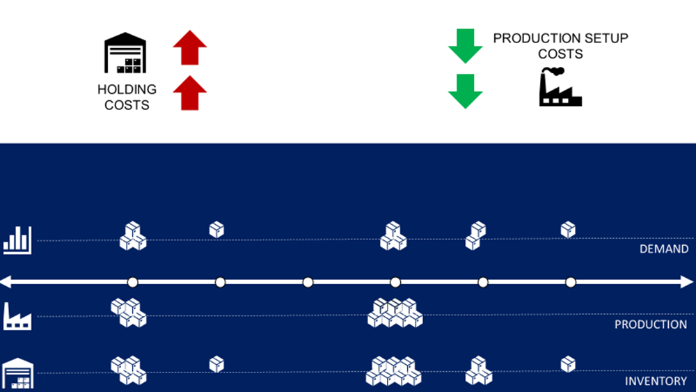
In this example, you build stock to minimise the number of setups

• Pros: only two production setups for the whole period
• Cons: a large stock on hand that increases the inventory costs

Conclusion

You need an optimisation algorithm to balance the two constraints.

Solution

Assumptions

Let us suppose that you receive a purchase order for the next 12 months with the quantities presented in the chart above.

• Set up cost: 500 $
• Holding cost: 1 $/unit/month
• Production cost per unit: 50 $/unit
• Units produced in month M can be shipped the same month
• Inventory costs are charged from the month m+1

Wagner-Whitin Algorithm

This problem can be seen as a generalisation of the economic order quantity model that takes into account that demand for the product varies over time.

Wagner and Whitin developed an algorithm for finding the optimal solution by dynamic programming.

The idea is to determine each month whether adding the current month's demand quantity to past months' orders is more economical than setting up a new production cycle.

Forward Calculation

Start at period 1:

• Calculate the total cost to satisfy the demand of month 1, D(1)

Period N:

• Calculate the total cost to satisfy the demand of month t, D(t)
• Look at all past orders (t=1 .. N) and find the cost for ordering for D(t) by adding the quantity to past orders D(t-1)
• Take the most economic option and go to t = N+1

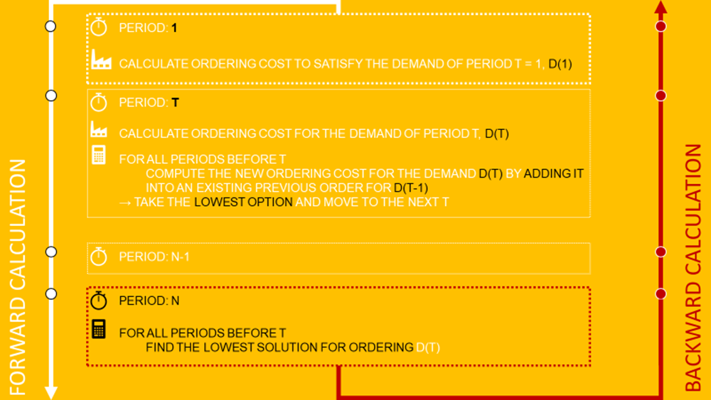
Backward Calculation

Start from period t = N and work backwards to find the lowest options to satisfy the demand of each D(t).

Results & Conclusion

Forward Calculation

You should export the results of the forward calculation using a table like the one below:

Let me take a few examples:

Period 1, if you produce for the

• First month demand only (D(1) = 200 units): 500$
• Two first months (D(1) + D(2) = 350 units): 650$

Backward Calculation

We can use the table above to visually verify the algorithm's output using the rules explained earlier.

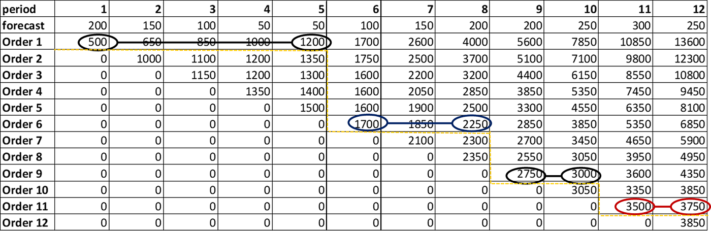
• Start with t = 12
  The cheapest solution is to produce the month 11 for D(11) + D(12)
• Continue with t = 10
  The cheapest solution is to produce the month 9 for D(9) + D(10)
• Continue with t = 8
  The cheapest solution is to produce the month 6 for D(6) + D(7) + D(8)
• Continue with t = 6
  The cheapest solution is to produce the month 1 for D(1) + D(2) + D(3) + D(4) + D(5) + D(6)

Final Solution

• Month 1: produce 550 units to meet the demand of the first 5 months
• Month 6: produce 450 units for months 6, 7 and 8
• Month 9: produce 450 units for months 9 and 10
• Month 11: produce 550 for months 11 and 12

Inventory Optimization

In the chart below, you can see that the inventory on hand (IOH) is very close to the demand forecast

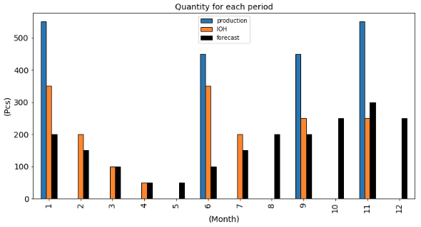
A great balance between inventory and set-up costs

In the chart below, you can follow the cumulative holding and set-up costs along the 12 months:

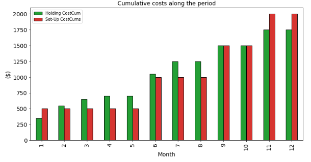
We can clearly see here how the algorithm is making the balance between inventory optimization and reducing the number of setups.

Implementation with Python

In the GitHub repository, you can find an implementation of this method from scratch using Python.

Using pandas functions to manipulate data frames, this method is easy to implement and works well for small datasets.

Have you heard about AI Agents?

For a customer in the automotive industry, we experimented with the usage of AI workflows to improve this tool.

The idea was to connect this algorithm to a mailbox that received purchase orders from the commercial team.

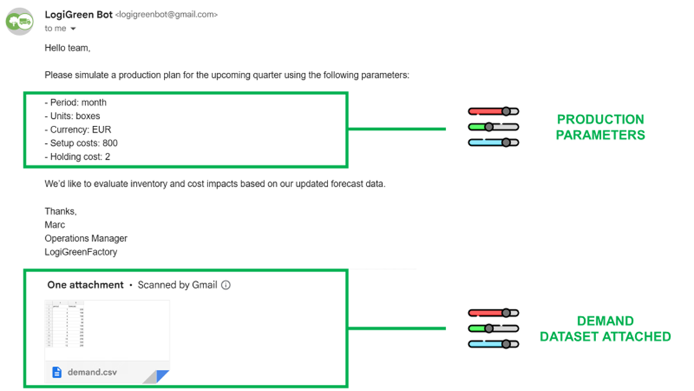
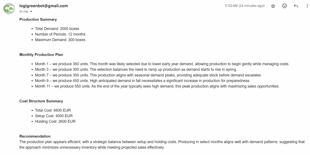
The agent can parse the email content, call the tool, and provide a reply.

For more details,

About Me

Let’s connect on LinkedIn and Twitter. I am a Supply Chain Engineer who is using data analytics to improve logistics operations and reduce costs.

If you’re looking for tailored consulting solutions to optimize your supply chain and meet sustainability goals, feel free to contact me.