Build and Deploy Your First Supply Chain App in 20 Minutes

In Supply Chain Management, it is easy to make an impact with your data science and analytics skills.

Even if data quality remains an issue most of the time, you can find opportunities to solve problems by providing insights to operational teams.

Operations Manager: "How many temporary workers should I recruit next to meet our workforce demand at the lowest cost?

When I was a Supply Chain Solution Manager in a logistics company, I learned data science by applying mathematical principles to solve operational problems in our warehouses.

It was very archaic.

I was running Python scripts or Jupyter notebooks on my machine and sharing the results with my colleagues.

Until I discovered Streamlit, which let me effortlessly package my models into web applications that I could easily deploy.

This is crucial for any supply chain process engineer or data scientist to learn how to productise analytics tools.

How to transform Python code into actionable insights?

In this article, I will show you how to transform a simulation model built in Jupyter Notebook into a fully functioning web application.

This exercise was part of a tutorial series on my YouTube Channel, in which we use Python to learn Inventory Management in Supply Chain.

You will learn how I took a core module written in Python scripts to build an interactive application with which you can:

• Simulate multiple inventory management rules
• Test several scenarios with different delivery lead times (LD in days), demand variability (sigma in pieces) and cycle time (T in days)

If you are not familiar with these concepts, you can still follow this tutorial, as I will briefly introduce them in the first section.

Or you can directly jump into the second section that focuses only on the creation and deployment of the app.

Note: This is an introductory tutorial to help you build and deploy your first app. If you need more challenging exercises, have a look at the case studies shared in the conclusion.

Inventory Management Simulation with Python

What is inventory management?

Most retailers I’ve worked with in Asia and Europe manage store orders with rule-based methods built into their ERPs.

When do you need to replenish your stores to avoid stock-outs?

These rules are usually implemented in an Enterprise Resource Planning (ERP) software that sends orders to a Warehouse Management System (WMS).

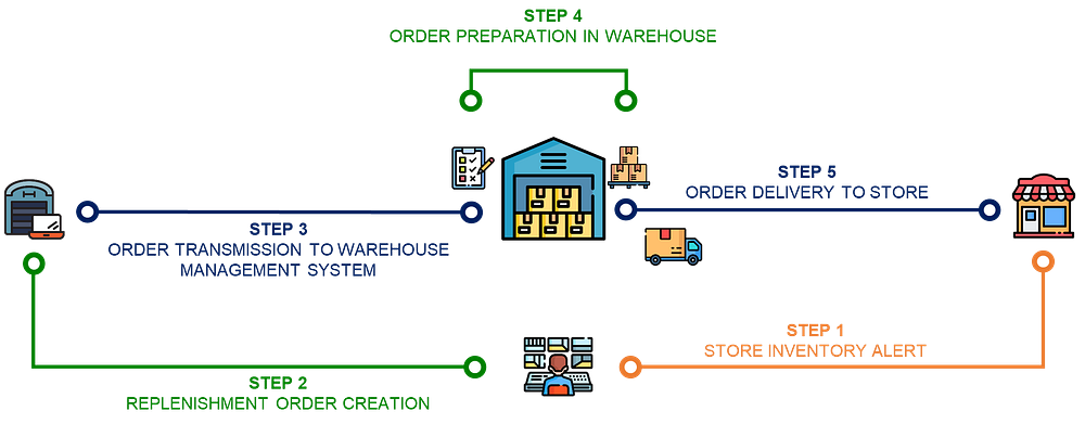
The goal is to develop a policy that minimises ordering, holding and shortage costs.

• Ordering Costs: fixed cost to place an order
• Holding Costs: variable costs required to keep your inventory (storage and capital costs)
• Shortage Costs: the costs of not having enough inventory to meet the customer demand (Lost Sales, Penalty)

We will act as data scientists in a retail company and assess the efficiency of the inventory team’s rules.

Logistics Director: "Samir, we need your support to understand why some stores face stockouts while other have too much inventory."

For that, we need a tool to simulate multiple scenarios and visualise the impact of key parameters on costs and stock availability.

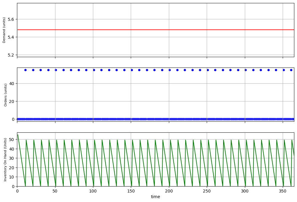
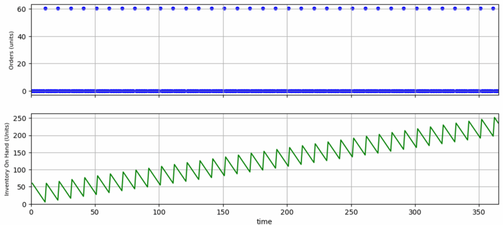
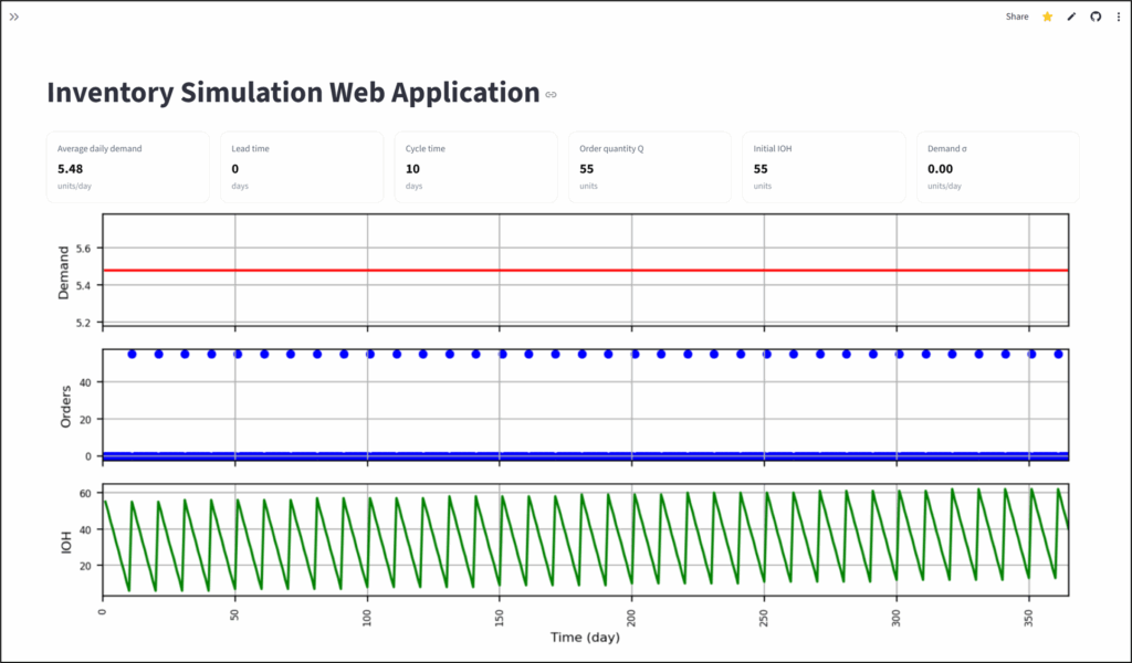
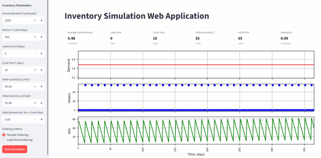
In the chart above, you have an example of a rule with:

• A uniform demand distribution (i.e., σ = 0)
  Every day, your store will sell the same number of items.
• A periodic review policy with T = 10 days
  You replenish the stores every 10 days.
• A delivery lead time of LD = 1 day.
  If you order today, you will receive the goods tomorrow.

As you can see in the green chart, your inventory on-hand (IOH) is always positive (i.e. you don't experience stock-outs).

1. What if you have a 3-day lead time?
2. What would be the impact of variability in the demand (σ > 0)?
3. Can we reduce the average inventory on hand?

To answer these questions, I developed a simulation model using Jupyter Notebook to generate visuals in a complete tutorial.

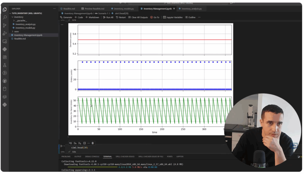
In this article, I will briefly introduce the core functions I built in this tutorial and show how we will reuse them in our Streamlit app.

Note: I will keep explanations high-level to focus on the Streamlit app. For details, you can watch the full video later.

Your Inventory Simulation Tool in a Jupyter Notebook

The results of this tutorial will serve as the core foundation of our Inventory Simulation Streamlit App.

The project structure is basic with two Python files (.py) and a Jupyter Notebook.

tuto_inventory /
├─ Inventory Management.ipynb
└─ inventory/
├─ init.py
├─ inventory_analysis.py
└─ inventory_models.py

In inventory_models.py, you can find a Pydantic class that contains all the input parameters for our simulation.

from typing import Optional, Literal
from pydantic import BaseModel, Field


class InventoryParams(BaseModel):
    """Base economic & demand parameters (deterministic daily demand)."""
    D: float = Field(2000, gt=0, description="Annual demand (units/year)")
    T_total: int = Field(365, ge=1, description="Days in horizon (usually 365)")
    LD: int = Field(0, ge=0, description="Lead time (days)")
    T: int = Field(10, ge=1, description="Cycle time (days)")
    Q: float = Field(0, ge=0, description="Order quantity (units)")
    initial_ioh: float = Field(0, description="Initial inventory on hand")
    sigma: float = Field(0, ge=0, description="Standard deviation of daily demand (units/day)")

These operational parameters cover

• Demand Distribution: the total demand D (pcs), our simulation horizon T_total (pcs) and the variability σ (pcs)
• Logistics Operations: with the delivery lead time LD (in days)
• Inventory rule parameters: including the cycle time T, order quantity Q and the initial inventory on hand initial_ioh

Based on these parameters, we want to simulate the impact on our distribution chain:

• Demand distribution: how many units were sold?
• Inventory On-Hand in green: how many units do we have in the store?
• Replenishment orders in blue: when and how much have we ordered?

In the example above, you see a simulation of a periodic review policy with a 10-day cycle time.

How did I generate these visuals?

These functions are simulated using the class InventorySimulation created in inventory_analysis.py.

class InventorySimulation:
    def __init__(self, 
                 params: InventoryParams):
        self.type = type
        self.D = params.D
        self.T_total = params.T_total
        self.LD = params.LD
        self.T = params.T
        self.Q = params.Q
        self.initial_ioh = params.initial_ioh
        self.sigma = params.sigma
        
        # # Demand per day (unit/day)
        self.D_day = self.D / self.T_total
        
        # Simulation dataframe
        self.sim = pd.DataFrame({'time': np.array(range(1, self.T_total+1))})

We start by initialising the input parameters for the functions:

• order() which represents a periodic ordering policy (you order Q units every T days)
• simulation_1() that calculates the impact of the demand (sales) and the ordering policy on the inventory on hand each day

class InventorySimulation:
    ''' [Beginning of the class] ''' 
    def order(self, t, T, Q, start_day=1):
        """Order Q starting at `start_day`, then every T days."""
        return Q if (t > start_day and ((t-start_day) % T) == 0) else 0
    def simulation_1(self):
        """Fixed-cycle ordering; lead time NOT compensated."""
        sim_1 = self.sim.copy()
        sim_1['demand'] = np.random.normal(self.D_day, self.sigma, self.T_total)
        T = int(self.T)
        Q = float(self.Q)
        sim_1['order'] = sim_1['time'].apply(lambda t: self.order(t, T, Q))
        LD = int(self.LD)
        sim_1['receipt'] = sim_1['order'].shift(LD, fill_value=0.0)
        # Inventory: iterative update to respect lead time
        ioh = [self.initial_ioh]
        for t in range(1, len(sim_1)):
            new_ioh = ioh[-1] - sim_1.loc[t, 'demand']
            new_ioh += sim_1.loc[t, 'receipt']
            ioh.append(new_ioh)
        sim_1['ioh'] = ioh
        for col in ['order', 'ioh', 'receipt']:
            sim_1[col] = np.rint(sim_1[col]).astype(int)
        return sim_1 

The function simulation_1() includes a mechanism that updates inventory on-hand based on store demand (sales) and supply (replenishment orders).

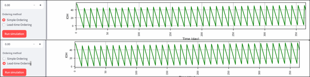
My goal for this tutorial was to start with two basic rules to explain what happens when you introduce a lead time, as shown below.

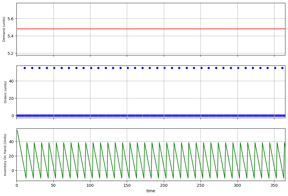
Stores experience stock-outs, as shown in the green chart.

Their on-hand inventory becomes negative due to late deliveries.

What can we do? Maybe increasing the order quantity Q?

This is what I tried in the tutorial; we discovered that this solution does not work.

These two scenarios highlighted the need for an improved ordering policy that compensates for lead times.

That is what we built in the second part of the tutorial with these two additional functions.

class InventorySimulation:
    ''' [Beginning of the class] ''' 

    def order_leadtime(self, t, T, Q, LD, start_day=1):
        return Q if (t > start_day and ((t-start_day + (LD-1)) % T) == 0) else 0

    def simulation_2(self, method: Optional[str] = "order_leadtime"):
        """Fixed-cycle ordering; lead time NOT compensated."""
        sim_1 = self.sim.copy()
        LD = int(self.LD)
        sim_1['demand'] = np.maximum(np.random.normal(self.D_day, self.sigma, self.T_total), 0)
        T = int(self.T)
        Q = float(self.Q)
        if method == "order_leadtime":
            sim_1['order'] = sim_1['time'].apply(lambda t: self.order_leadtime(t, T, Q, LD))
        else:
            sim_1['order'] = sim_1['time'].apply(lambda t: self.order(t, T, Q))
        sim_1['receipt'] = sim_1['order'].shift(LD, fill_value=0.0)
        # Inventory: iterative update to respect lead time
        ioh = [self.initial_ioh]
        for t in range(1, len(sim_1)):
            new_ioh = ioh[-1] - sim_1.loc[t, 'demand']
            new_ioh += sim_1.loc[t, 'receipt']
            ioh.append(new_ioh)
        sim_1['ioh'] = ioh
        for col in ['order', 'ioh', 'receipt']:
            sim_1[col] = np.rint(sim_1[col]).astype(int)
        return sim_1   

The idea is quite simple.

In practice, that means inventory planners must create replenishment orders at day = T - LD to compensate for the lead time.

This ensures stores receive their goods on day = T as shown in the chart above.

At the end of this tutorial, we had a complete simulation tool that lets you test any scenario to become familiar with inventory management rules.

If you need more clarification, you can find detailed explanations in this step-by-step YouTube tutorial:

However, I was not satisfied with the result.

Why do we need to package this in a web application?

Productising This Simulation Tool

As you can see in the video, I manually changed the parameters in the Jupyter notebook to test different scenarios.

This is somewhat normal for data scientists like us.

But, would you imagine our Logistics Director opening a Jupyter Notebook in VS Code to test the different scenarios?

We need to productise this tool so anyone can access it without requiring programming or data science skills.

Good news, 70% of the job is done as we have the core modules.

In the next section, I will explain how we can package this in a user-friendly analytics product.

Create your Inventory Simulation App using Streamlit

In this section, we will create a single-page Streamlit App based on the core module from the first tutorial.

You can start by cloning this repository that contains the core simulation, including inventory_models.py and inventory_analysis.py.

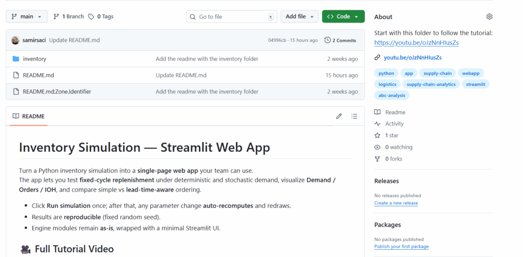
With this repository on your local machine, you can follow the tutorial and end up with a deployed app like this one:

Let's start!

Project Setup

The first step is to create a local Python environment for the project.

For that, I advise you to use the package manager uv:

# Create a virtual environment and activate it
uv init
uv venv
source .venv/bin/activate

# Install
uv pip install -r requirements.txt

It will install the libraries listed in the requirements file:

streamlit>=1.37
pandas>=2.0
numpy>=1.24
matplotlib>=3.7
pydantic>=2.0

We include Streamlit, Pydantic, and libraries for data manipulation (numpy, pandas) and for generating visuals (matplotlib).

Now you are ready to build your app.

Create your Streamlit Page

Create a Python file that you call: app.py

import numpy as np
import matplotlib.pyplot as plt
import streamlit as st
from inventory.inventory_models import InventoryParams
from inventory.inventory_analysis import InventorySimulation
seed = 1991
np.random.seed(seed)

st.set_page_config(page_title="Inventory Simulation – Streamlit", layout="wide")

In this file, we start by:

• Importing the libraries installed and the analysis module with its Pydantic class for the input parameters
• Defining a seed for random distribution generation that will be used to generate a variable demand

Then we start to create the page with st.set_page_config(), in which we include as parameters:

• page_title: the title of the web page of your app
• layout: an option to set the layout of the page

By setting the parameter layout to "wide", we ensure the page is wide by default.

You can run your app now,

streamlit run app.py

After running this command, your app can be opened using the local URL shared in your terminal:

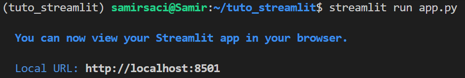
After loading, what you have is this blank page:

Congratulations, you have run your app!

If you face any issues at this stage, please check that:

• The local Python environment is set up properly
• You have installed all the libraries inside the requirements file

Now we can start building our Inventory Management App.

A Sidebar with Inventory Management Parameters

Do you remember the Pydantic class we have defined in inventory_models.py?

They will serve as our input parameters for the app, and we will display them in a Streamlit sidebar.

with st.sidebar:
    st.markdown("**Inventory Parameters**")
    D = st.number_input("Annual demand D (units/year)", min_value=1, value=2000, step=50)
    T_total = st.number_input("Horizon T_total (days)", min_value=1, value=365, step=1)
    LD = st.number_input("Lead time LD (days)", min_value=0, value=0, step=1)
    T = st.number_input("Cycle time T (days)", min_value=1, value=10, step=1)
    Q = st.number_input("Order quantity Q (units)", min_value=0.0, value=55.0, step=10.0, format="%.2f")
    initial_ioh = st.number_input("Initial inventory on hand", min_value=0.0, value=55.0, step=1.0, format="%.2f")
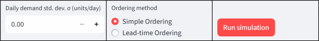
    sigma = st.number_input("Daily demand std. dev. σ (units/day)", min_value=0.0, value=0.0, step=0.5, format="%.2f")
    method = st.radio(
        "Ordering method",
        options=["Simple Ordering", "Lead-time Ordering"],
        index=0
    )
    method_key = "order_leadtime" if method.startswith("Lead-time") else "order"
    
    run = st.button("Run simulation", type="primary")
    if run:
        st.session_state.has_run = True

In this sidebar, we include:

• A title using st.markdown()
• Number Input fields for all the parameters with their minimum, default, and incremental step values
• A radio button to select the ordering method (considering or not lead time)
• A button to start the first simulation

Before this block, we should add a session state variable:

if "has_run" not in st.session_state:
    st.session_state.has_run = False

This boolean indicates whether the user has already clicked the simulation button.

If that's the case, the app will automatically rerun all calculations whenever the user changes a parameter.

Great, now you app.py should look like this:

import numpy as np
import matplotlib.pyplot as plt
import streamlit as st
from inventory.inventory_models import InventoryParams
from inventory.inventory_analysis import InventorySimulation
seed = 1991
np.random.seed(seed)

st.set_page_config(page_title="Inventory Simulation – Streamlit", layout="wide")

if "has_run" not in st.session_state:
    st.session_state.has_run = False

with st.sidebar:

    st.markdown("**Inventory Parameters**")
    D = st.number_input("Annual demand D (units/year)", min_value=1, value=2000, step=50)
    T_total = st.number_input("Horizon T_total (days)", min_value=1, value=365, step=1)
    LD = st.number_input("Lead time LD (days)", min_value=0, value=0, step=1)
    T = st.number_input("Cycle time T (days)", min_value=1, value=10, step=1)
    Q = st.number_input("Order quantity Q (units)", min_value=0.0, value=55.0, step=10.0, format="%.2f")
    initial_ioh = st.number_input("Initial inventory on hand", min_value=0.0, value=55.0, step=1.0, format="%.2f")
    sigma = st.number_input("Daily demand std. dev. σ (units/day)", min_value=0.0, value=0.0, step=0.5, format="%.2f")
    method = st.radio(
        "Ordering method",
        options=["Simple Ordering", "Lead-time Ordering"],
        index=0
    )
    method_key = "order_leadtime" if method.startswith("Lead-time") else "order"
    
    run = st.button("Run simulation", type="primary")
    if run:
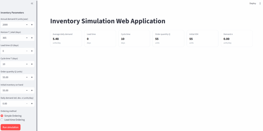
        st.session_state.has_run = True

You can have a look at your app, normally the window should look like this after a refresh:

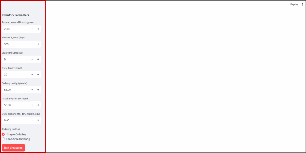
On the left, you have your sidebar that we just created.

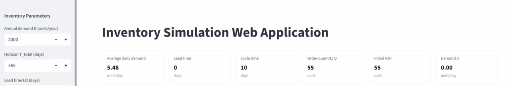
Then, for aesthetics and user experience, I want to add a title and a reminder of the parameters used.

Why do I want to remind the parameters used?

On the top-left side of the window, you have a button to hide the side panel, as shown below.

This helps users to have more space to show the visual.

However, the input parameters will be hidden.

Therefore, we need to add a reminder at the top.

st.title("Inventory Simulation Web Application")
# Selected Input Parameters
D_day = D / T_total
st.markdown("""
<style>
.quick-card{padding:.9rem 1rem;border:1px solid #eaeaea;border-radius:12px;background:#fff;box-shadow:0 1px 2px rgba(0,0,0,.03)}
.quick-card .label{font-size:.85rem;color:#5f6b7a;margin:0}
.quick-card .value{font-size:1.25rem;font-weight:700;margin:.15rem 0 0 0;color:#111}
.quick-card .unit{font-size:.8rem;color:#8a95a3;margin:0}
</style>
""", unsafe_allow_html=True)

def quick_card(label, value, unit=""):
    unit_html = f'<p class="unit">{unit}</p>' if unit else ""
    st.markdown(f'<div class="quick-card"><p class="label">{label}</p><p class="value">{value}</p>{unit_html}</div>', unsafe_allow_html=True)

In the piece of code above, I have introduced :

• CSS styling embedded in Streamlit to create cards
• The function quick_card will create a card for each parameter using its label, value and units

Then we can generate these cards in the same row using the streamlit object st.columns().

c1, c2, c3, c4, c5, c6 = st.columns(6)
with c1:
    quick_card("Average daily demand", f"{D_day:,.2f}", "units/day")
with c2:
    quick_card("Lead time", f"{LD}", "days")
with c3:
    quick_card("Cycle time", f"{T}", "days")
with c4:
    quick_card("Order quantity Q", f"{Q:,.0f}", "units")
with c5:
    quick_card("Initial IOH", f"{initial_ioh:,.0f}", "units")
with c6:
    quick_card("Demand σ", f"{sigma:.2f}", "units/day")

The first line defines the six columns in which we place the cards using the quick_card function.

We can move on to the interesting part: integrating the simulation tool into the app.

Any question or blocking at this step? You can use the comment section of the video, I'll try my best to answer promptly.

Integrating the inventory simulation module in the Streamlit App

We can now start working on the main page.

Let us imagine that our Logistics Director arrives on the page, selects the different parameters and clicks on "Run Simulation".

This should trigger the simulation module:

if st.session_state.has_run:
    params = InventoryParams(
        D=float(D),
        T_total=int(T_total),
        LD=int(LD),
        T=int(T),
        Q=float(Q),
        initial_ioh=float(initial_ioh),
        sigma=float(sigma)
    )

    sim_engine = InventorySimulation(params)

In this short piece of code, we do many things:

• We build the input parameter object using the Pydantic class from inventory_models.py
  This ensures every value (demand, lead time, review period, sigma…) has the correct data type before running the simulation.
• We create the simulation engine InventorySimulation class from inventory_analysis.py
  This class contains all the inventory logic I developed in the first tutorial.

Nothing will change on the user interface.

We can now start to define the computation part.

if st.session_state.has_run:
    ''' [Previous block introduced above]'''
    if method_key == "order_leadtime":
        df = sim_engine.simulation_2(method="order_leadtime")
    elif method_key == "order":
        df = sim_engine.simulation_2(method="order")
    else:
        df = sim_engine.simulation_1()

    # Calculate key parameters that will be shown below the visual
    stockouts = (df["ioh"] < 0).sum()
    min_ioh = df["ioh"].min()
    avg_ioh = df["ioh"].mean()

First, we select the correct ordering method.

Depending on the ordering rule chosen in the radio button of the sidebar, we call the appropriate simulation method:

• method="order": is the initial method that I showed you, which failed to keep a stable inventory when I added a lead time
• method="order_leadtime": is the improved method that orders at day = T - LD

The results, stored in the pandas dataframe, df are used to compute key indicators such as the number of stockouts and the minimum and maximum inventory levels.

Now that we have simulation results available, let's create our visuals.

Create Inventory Simulation Visuals on Streamlit

If you followed the video version of this tutorial, you probably noticed that I copied and pasted the code from the notebook created in the first tutorial.

if st.session_state.has_run:
    '''[Previous Blocks introduced above]'''
    # Plot
    fig, axes = plt.subplots(3, 1, figsize=(9, 4), sharex=True)  # ↓ from (12, 8) to (9, 5)
    # Demand
    df.plot(x='time', y='demand', ax=axes[0], color='r', legend=False, grid=True)
    axes[0].set_ylabel("Demand", fontsize=8)
    # Orders
    df.plot.scatter(x='time', y='order', ax=axes[1], color='b')
    axes[1].set_ylabel("Orders", fontsize=8); axes[1].grid(True)
    # IOH
    df.plot(x='time', y='ioh', ax=axes[2], color='g', legend=False, grid=True)
    axes[2].set_ylabel("IOH", fontsize=8); axes[2].set_xlabel("Time (day)", fontsize=8)
    # Common x formatting
    axes[2].set_xlim(0, int(df["time"].max()))
    for ax in axes:
        ax.tick_params(axis='x', rotation=90, labelsize=6)
        ax.tick_params(axis='y', labelsize=6)
    plt.tight_layout()

Indeed, the same visual code that you use to prototype in your Notebooks will work in your app.

The only difference is that instead of using plt.show(), you conclude the section with:

st.pyplot(fig, clear_figure=True, use_container_width=True)  

Streamlit needs to explicitly control of the rendering using

• fig the Matplotlib figure you created earlier.
• clear_figure=True This parameter clears the figure from memory after rendering to prevent duplicate plots when parameters are updated.
• use_container_width=True to make the chart automatically resize to the width of the Streamlit page

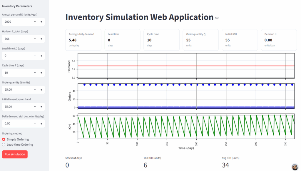
At this stage, normally, you have this on your app:

If you try to change any parameter, for example, change the ordering method, you will see the visual automatically updated.

What is remaining?

As a bonus, I added a section to help you discover additional functionalities of streamlit.

if st.session_state.has_run:
    '''[Previous Blocks introduced above]'''
    # Key parameters presented below the visual
    kpi_cols = st.columns(3)
    kpi_cols[0].metric("Stockout days", f"{stockouts}")
    kpi_cols[1].metric("Min IOH (units)", f"{min_ioh:,.0f}")
    kpi_cols[2].metric("Avg IOH (units)", f"{avg_ioh:,.0f}")

    # Message of information
    st.success("Simulation completed.")

In addition to the columns that we already defined in the previous section, we have:

• metric() that generates a clean and built-in Streamlit card
  Unlike my custom card, you don't need CSS here.
• st.success() to display a green success banner to notify the user that the results have been updated.

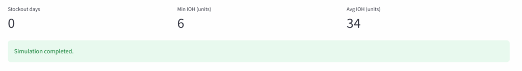
This is the cherry on the cake that we needed to conclude this app.

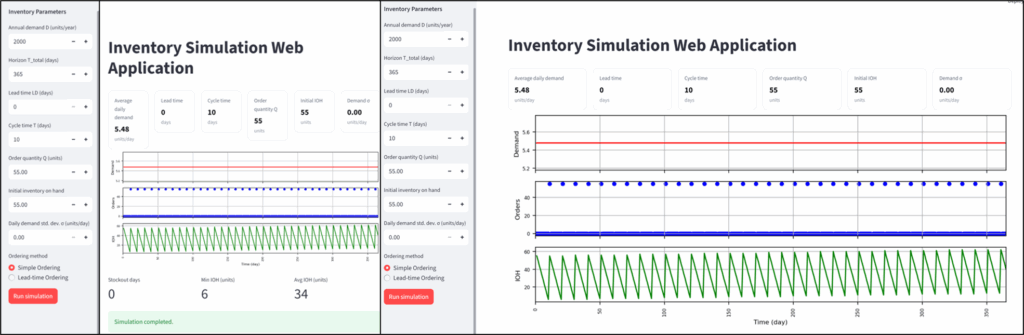
You now have a complete app that automatically generates visuals and easily tests scenarios, working on your machine.

What about our Logistics Director? How he can use it?

Let me show you how to deploy it for free on Streamlit Community Cloud easily.

Deploy your App on Streamlit Community

First, you need to push your code to GitHub, as I did here: GitHub Repository.

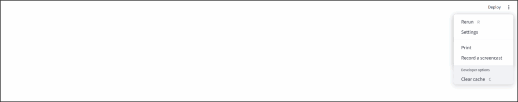
Then you go to the top right of your app, and you click on Deploy.

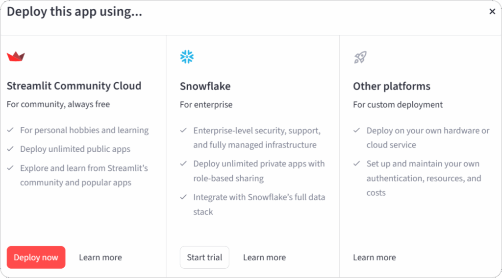
Then click Deploy now and follow the steps to grant Streamlit access to your GitHub account (Streamlit will automatically detect that you have pushed your code to GitHub).

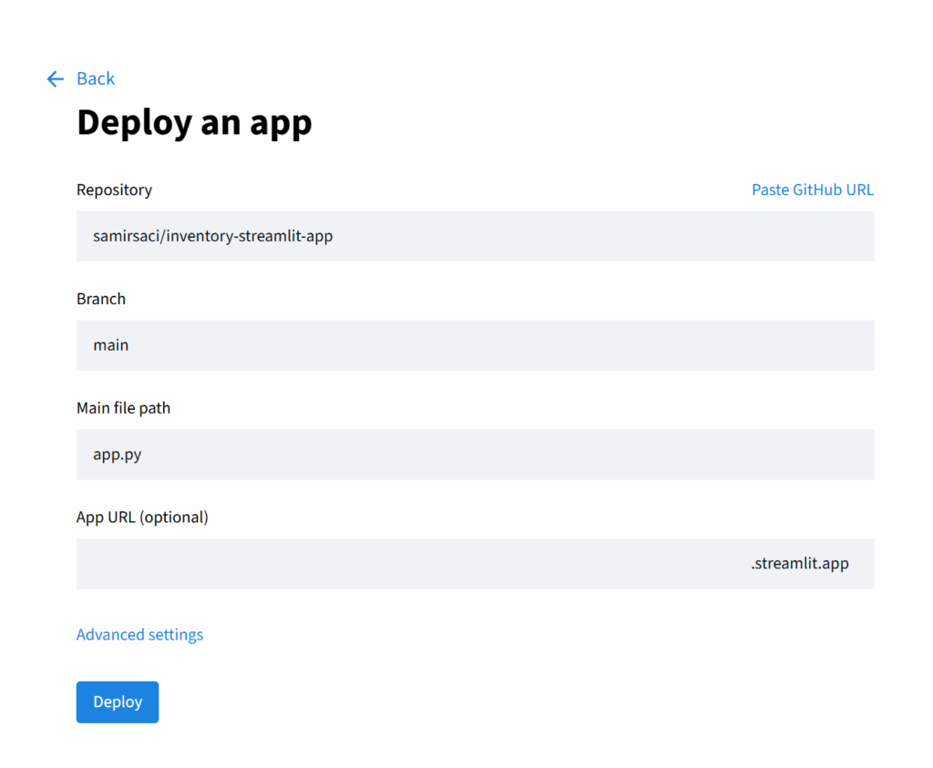
You can create a custom URL: mine is supplyscience.

After clicking Deploy, Streamlit will redirect you to the deployed app.

Congratulations, you have deployed your first Supply Chain Analytics Streamlit App!

Feel free to check the complete tutorial.

Feel free to use the comment to ask your questions or share what you deployed on Streamlit.

Conclusion

I designed this tutorial for the version of myself from 2018.

At the time, I knew enough Python and analytics to build optimisation and simulation tools for my colleagues, but I did not yet know how to turn them into real products.

This tutorial is the first step in your journey toward industrialising analytics solutions.

What you built here is probably not production-ready, but it is a functional app that you can share with our Logistics Director.

Do you need inspiration for other applications?

How to Complete this App?

Now that you have the playbook for deploying Supply Chain Analytics applications, you likely want to improve the application by adding more models.

I have a suggestion for you.

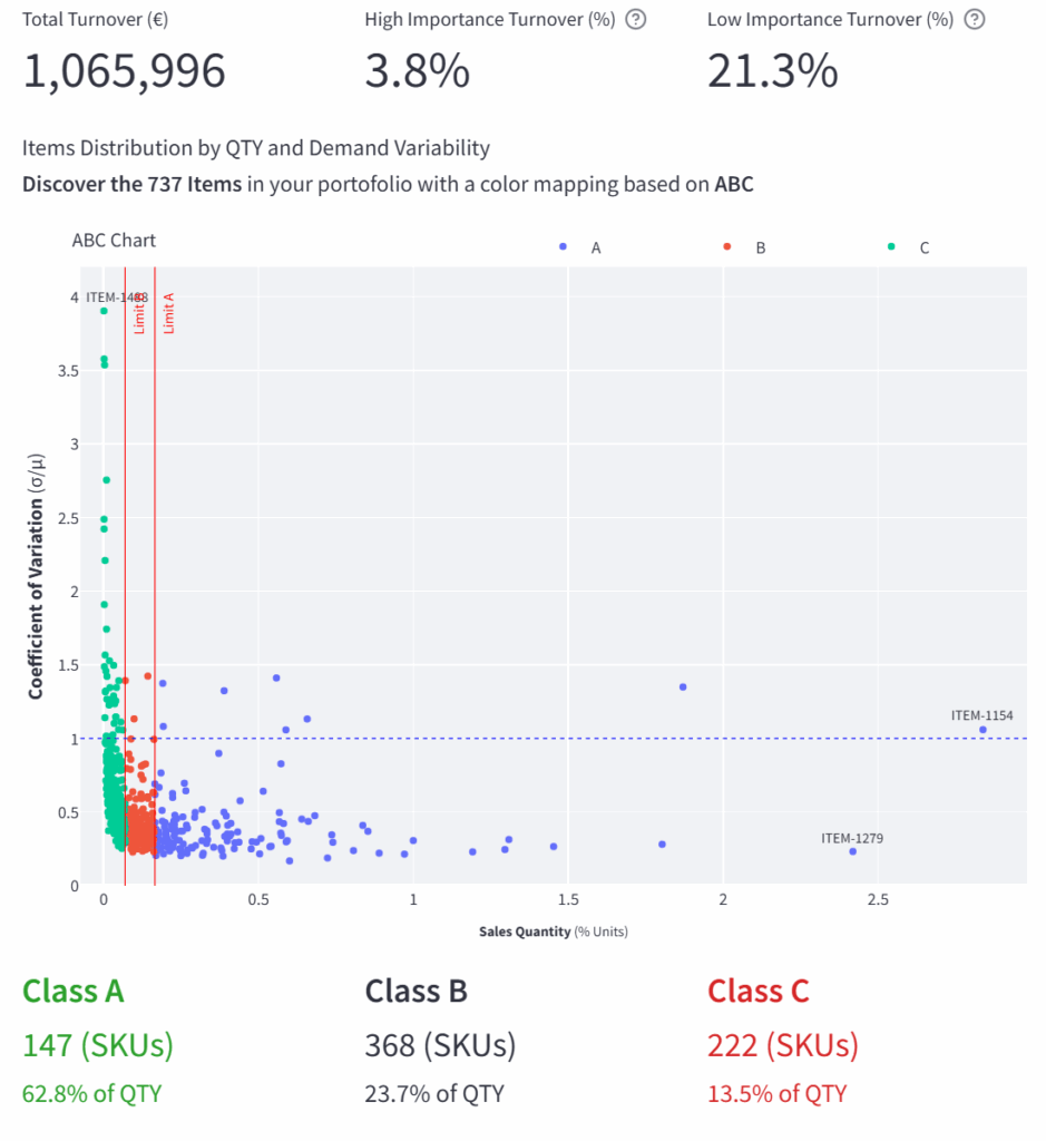
You can follow this step-by-step tutorial to implement Product Segmentation with Pareto Analysis and ABC Chart.

You will learn how to deploy strategic visuals, such as the ABC XYZ, to help retail companies manage their inventory.

This can be easily implemented on the second page of the app that you just deployed.

If needed, I can work on another article focusing on this solution!

Tired of inventory management?

You can find 80+ case studies of AI & analytics products to support Supply Chain Optimisation, Business Profitability and Process Automation in this cheat sheet.

For most of the case studies, published in Towards Data Science, you can find the source code that can be implemented in a Streamlit app.

About Me

Let’s connect on LinkedIn and Twitter. I am a Supply Chain Engineer who uses data analytics to improve logistics operations and reduce costs.

For consulting or advice on analytics and sustainable supply chain transformation, feel free to contact me via Logigreen Consulting.

If you are interested in Data Analytics and Supply Chain, look at my website.

Samir Saci | Data Science & Productivity